Effects of stock rebuilding – A computable general equilibrium analysis for a mackerel fishery in Korea

Globally, many fish stocks are depleted mainly due to overfishing. One reason for the overfishing is an increasing human demand for fish. The volume of aggregate fish demand (live weight) increased by 62% (from 93.6 to 152 million tons) during the period from 1998 to 2018. The global fish demand is projected to double by 2050¹. Depletion of fish stocks poses a serious threat to the oceans and jeopardizes sustainable fisheries and the social and economic well-being of fishing-dependent communities worldwide. The proportion of fishery stocks within biologically sustainable levels was 90% in 1974 and declined to 64.6% in 2019. In contrast, the proportion of stocks within biologically unsustainable levels has been increasing from 10% in 1974 to 35.4% in 2019. (https://www.fao.org/3/cc0461en/online/sofia/2022/status-of-fishery-esources.html#note-1_13, accessed June 27, 2023). To address this problem, governments have exerted efforts to rebuild the depleted stocks and some of them were successful^2,3. In some cases, however, governments hesitate to implement a stock rebuilding plan due to its short-term negative economic impacts although the long-term positive effects may more than offset the negative impacts^2,4,5.

Extant studies of the potential economic effects of stock rebuilding focus on either national fisheries^6,7,8, multi-national fisheries in a continent⁹, or global fisheries¹⁰. Although results from these studies will be useful for formulating national or global fishery management policies to boost fish stocks, they will provide little insight regarding the sub-national (regional or local) economic impacts of a rebuilding program for a sub-national fishery. Furthermore, the economic models used in these studies are either partial equilibrium models^11,12 that ignore the general equilibrium effects occurring outside the fishery being rebuilt or fixed-price models, such as input–output (IO) models^6,8 which do not allow substitution effects, and therefore, fail to evaluate the welfare effects.

There are a number of studies that used general equilibrium models for the analysis of fisheries. For instance, the relationship between international trade and open-access renewable resources (fisheries) was examined using a two-sector general equilibrium model¹³. A dynamic CGE model was linked with ecological general equilibrium models for Alaska pollock fisheries¹⁴. The rationalization for a fishing community in the western Philippines was investigated using a CGE model¹⁵. A more recent study examined the regional welfare effects of transitioning from regulated open access to a rationalized fishery for a sub-national region in Korea¹⁶. None of the previous studies assessed the sub-national economic impacts of a stock rebuilding program for a sub-national fishery using a general equilibrium framework. Although results from these studies provide some implications for the recovery of fish stock, they did not evaluate the specific stock rebuilding programs such as those addressed in our study.

To address this hiatus in the literature, we use a CGE model to analyze the sub-national (local) impacts of rebuilding the depleted Chub mackerel (Scomber japonicus) (hereafter ‘mackerel’) harvested in the waters off Busan, Korea. When assessing the economy-wide effects of a fishery management policy such as a stock rebuilding policy, it is important to use a general equilibrium approach. The reason is that the approach accounts for the interactions between the fishing sector and non-fishing sectors in an economy. For example, if a fishery management policy is implemented, it will alter the levels of harvest and effort. The change in the harvest level leads to a change in the fishing sector’s demand for intermediate inputs from non-fishing sectors, resulting in a change in the production in the non-fishing sectors. This will lead to a change in the prices of the commodities that the non-fishing sectors produce. Additionally, the change in the level of effort will affect the supply of the factors of production available to the non-fishing sectors, leading to a change in the factor prices. The changes in the factor and commodity prices will, in turn, have feedback effects on the fishing sector, affecting the fishermen’s decision-making which depends on the commodity and factor prices.

When rebuilding a depleted fish stock, governments worldwide often try to achieve the target level of biomass corresponding to maximum sustainable yield (MSY); that is, Bmsy. The present study examines the economic and welfare effects of rebuilding the mackerel stock by reducing its harvest (lowering its TAC) to reach its Bmsy. One policy option for rebuilding the fish stock will be to reduce exogenously the TAC by a certain percentage assuming that the industry exhausts the full TAC, and to maintain the reduced TAC until the goal (Bmsy) is reached. We evaluate the economic and welfare effects of this type of policy option using a recursive dynamic CGE model. In the model, fishermen maximize in each period (year) their profits by adjusting (substituting between) the inputs used in fishing (labor, capital, and intermediate inputs) given (i) the harvest (TAC) level, (ii) the stock level, (iii) the effort level, and (iv) the factor and commodity prices. Fixing the harvest and stock levels means that the effort level is also fixed. See the fish harvest function used in our study (Eq. (A.1) in Supplementary Information, Section A). With fixed effort, the fishermen’s problem is to choose the input levels to maximize their profits. See Eq. (A.3) in Supplementary Information, Section A, for the effort function. Specifically, we incrementally increase by 5% the size of the TAC reduction by up to 100%, yielding a total of 20 different scenarios, each scenario representing a percentage reduction in the TAC. In each scenario, we maintain the lowered level of harvest until the stock level reaches Bmsy and fix the TAC at MSY afterwards.

The contribution of this study is that it develops the first regional CGE model to assess the regional economic and welfare effects of fish stock rebuilding. By conducting this study, we attempt to answer the following questions from a general equilibrium perspective. First, which of the 20 scenarios performs the best in terms of the three criteria—the mackerel sector’s resource rent, its value-added, and the aggregate regional welfare? Second, are there any trade-offs between ecological and economic benefits generated from harvest reductions in different magnitudes during the stock rebuilding period?

Chub mackerel (Scomber japonicus) (hereafter, ‘mackerel’) inhabit warm or tropical waters, including offshore and coastal waters of Korea¹⁷. Mackerel is one of the major species harvested in Korean wild fisheries and is a Korean favorite together with anchovy and squid¹⁸. In 2020, mackerel production was 77,401 tons, comprising about 11% of the total fish harvest from wild fisheries. In the same year, the ex-vessel revenue from mackerel catch totaled about 163,600 million Korean Won (KRW), or US$138.6 million (https://data.worldbank.org/indicator/PA.NUS.FCRF?end=2021&locations=KR&start=1995.

Accessed Oct. 31, 2022). This value is the fourth largest total ex-vessel revenue, following those of hairtail, anchovy, and yellow croaker harvests, and it accounts for about 7% of total ex-vessel revenue from wild fisheries¹⁹. Large purse seines catch a large fraction (85.8%, 66,444 tons) of the total mackerel harvest, followed by set nets (3.4% or 2644 tons), small purse seine (2.7% or 2057 tons), offshore gillnets (2.2% or 1689 tons), and large pair-trawls (2.1% or 1634 tons)¹⁹. Busan is where the majority of the mackerel caught in Korean waters is landed. In 2021, Busan accounts for 83% of the total mackerel catch from Korean waters.

In 1970, mackerel production was 38,256 tons. Since then, it has grown steadily until 1996, when it peaked at 415,003 tons. Since then it has been decreasing because of the reduced fish population from overexploitation¹⁹. The stock declined from 1,263,316 tons in 1970 to 442,660 tons in 2020²⁰. The level of stock in 2020 (442,660 tons) is 61% of its Bmsy (729,751 tons), and it concluded that the stock is overfished. This has prompted the Korean government to introduce various types of regulations. Besides the TAC system introduced for fisheries in 1999, it prohibits mackerel harvest for a month between April 1 and June 30 and sets a size limit of the fish at 21 cm²⁰. Now the government is considering rebuilding the stock by reducing the catch (TAC).

An earlier study of the effects of recovering fish stock used numerical models for moderate- and long-lived stocks¹¹. The study showed that, depending on the stock productivity and the discount rate, the economic benefits of the rebuilding plan can increase substantially if the rebuilding timeframe is extended. Another study tested whether closed fishing seasons increase the annual reproductive output of limpet (Cymbula granatina)²¹. The study found that a closed fishing season during the breeding period does not increase the reproductive output, having only marginal effects on yield if the total annual fishing effort remains the same. It found, however, that for the species that are disturbed by fishing or become vulnerable to fishing because they aggregate to breed, a closed season substantially increases the reproductive output during the breeding period. An input–output (IO) study found that achieving MEY would generate an overall reduction in the net economic benefit in the short term but a long-term net economic benefit to society⁶.

A dynamic bioeconomic optimization model, which explicitly accounts for the economics, management, and ecology of size-structured exploited fish populations, was used to find that rebuilding fisheries generates considerable economic gains while the magnitudes of the gains vary across fisheries¹². Using global databases, the research found that rebuilding the global marine fisheries would generate a net gain in resource rent of US$600 to US$1400 billion in present value over 50 years after rebuilding if the governments invest about US$203 billion in present value¹⁰. The research also found that it would take 12 years after the implementation of the rebuilding for the benefits to exceed the cost. A dynamic general equilibrium model was used to assess the economic consequences of rebuilding fish stock in the Mediterranean Sea in the EU and find that all aggregate results (e.g., results for gross value-added) improve if the stock rebuilding strategy is followed⁷.

A more recent study investigated the effects of four future exploitation scenarios for European fisheries and found that if 50–80% of the maximum sustainable yield is caught, the stocks will be rebuilt, which will lead to higher catches and profits than their current levels⁹. A research was conducted to assess the economic effects of rebuilding six depleted Canadian fish stocks under different biological and management scenarios and found that for five of the six fish stocks, the long-term economic gains from rebuilding would be 11 times and 5 times above the status quo, respectively, under the most and least optimistic scenarios⁸. Results from this research suggest that it is worthwhile to invest in rebuilding the stocks because the long-term economic benefits exceed the short-term costs of rebuilding.

We conduct a number of simulations, including baseline simulation and sensitivity analyses. The Korean government is assumed to recover the depleted mackerel stock to its Bmsy by reducing the harvest (TAC). To conduct baseline simulation, we first solve our CGE model for 30 years without any change in the TAC, producing a sequence of 30 benchmark solutions, each corresponding to each of the 30 years. Next, we lower the TAC by 5% in the base year and maintain the lowered TAC until the level of the stock reaches the target level (Bmsy) when solving the CGE model for 30 years. We then incrementally increase the size of the TAC reduction by 5% up to 100%, resulting in a total of 20 different scenarios (sequences) of 30 counterfactual solutions with each scenario representing a percentage reduction in the TAC. When we lower the TAC by a certain percentage, we maintain the lowered level until the stock level reaches the target level when solving the CGE model for 30 years. In all the scenarios, when the target stock level is reached, the TAC is fixed at MSY afterwards.

We solve the model for 30 years because, by the 30th year, all the endogenous variables approach their steady-state levels. Finally, we compute the effects (including welfare effects) of the stock rebuilding by comparing the results from each of the 20 different scenarios of counterfactual solutions with those from the benchmark solutions. We calculate the sum of the stream, over 30 years, of the present discounted values (SSPDV) of the three different measures of the benefits of the stock rebuilding—(i) the change in the mackerel sector’s rent (profit), (ii) the change in the sector’s value-added and (iii) the aggregate welfare change, as well as the effects on other variables.

In addition, we conduct sensitivity analyses for various parameters or assumptions. These parameters include the intrinsic growth rate of the stock, the initial ratio of the biomass to its carrying capacity, discount rate, the elasticities in import supply and export demand, the elasticities of substitution in the two different levels of the Armington function and CET function, the elasticities of substitution in the multi-level production and household consumption functions, and factor mobility. The parameter values used to conduct sensitivity analyses are presented in Supplementary Information, Section C, Supplementary Table C.4.

To illustrate how some of the important endogenous variables change over time because of the rebuilding plan, we first present, as an example, the results from a 10% reduction in the TAC, which is part of the baseline simulation, for the endogenous variables. Next, we present the sequence of the effects from all 20 different scenarios. Using the baseline values of elasticities (Supplementary Information, Section C, Supplementary Table C.3) and the other parameters calibrated with the elasticities, we solve the model with the TAC reduced by 10%. The reduced level persists until Bmsy is reached. We find that it takes 12 years before the Bmsy is reached. Thus, from the 13th year, we set the TAC at the level (MSY) corresponding to the Bmsy.

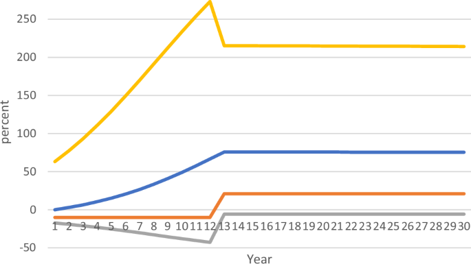
Table 1 and Figs. 1–3 present the effects on selected variables obtained from the 10% cut in TAC. The 10% cut leads to a decrease in the effort by 17.3% (Table 1, Fig. 2) and a rise in the fish price by 1.52% (Fig. 1) in the first year. Although the harvest is reduced (Fig. 2), the dramatic decrease in effort, along with a modest increase in the fish price, contributes to a substantial increase in the rent (Fig. 2); resource rent increases by 63.2% in the first year. Accordingly, value-added in the mackerel sector does not decrease as much as the mackerel harvest in terms of percent change. It decreases by only 3.8% (Table 1).

Percent change in fish price (10% cut in TAC).

Full size image

Percent change in biomass, harvest, effort, and rent (10% cut in TAC).

Full size image

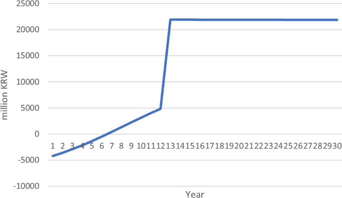
Aggregate welfare change (10% cut in TAC).

Full size image

The rise in the fish price induces mackerel consumers and processors in the region to substitute the cheaper imported mackerel for the regionally produced version. Domestic and foreign imports of mackerel increased by 7.8% and 0.4% in the first year (Table 1), respectively. In addition, due to the higher fish prices in the region, the fish producers in the region increase their supply to the regional market, reducing their supply to export markets. Domestic and foreign exports of mackerel shrank by 13.3% and 15.1%, respectively, in the first year. The aggregate welfare declined by 0.008% in the first year (Table 1, Fig. 3).

Reduction in TAC in the first 12 years leads to increased biomass (Fig. 2). In the 15th year, the mackerel biomass increases by 75.7% (Table 1) compared to its pre-policy (pre-rebuilding) level. In the same year, due to the higher biomass, harvest increases by 21.1%, causing the price to drop by 2.5% compared to its pre-policy level. Despite the price drop, the significant increase in the harvest coupled with a decrease in effort (5.8%) and the wage rate (not shown) contributes to a substantial increase in rent (215.1%) and value-added (31.4%). The cheaper price of mackerel induces the fish producers to increase their exports to both domestic regions and foreign countries while causing a reduction in Busan’s mackerel imports from the two sources (origins) of the commodity. The aggregate welfare increases by 0.04% (or by 21,903.0 million KRW, Fig. 3) in the 15th year.

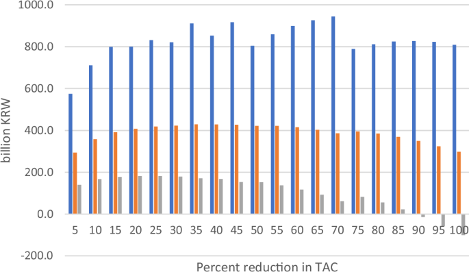
We found that all the variables start to approach a new steady state from year 15 and that the results for year 30 are not noticeably different from those for year 15 (see also Figs. 1–3). The sum of the stream of the present discounted values (SSPDV) over the 30 years of the increases in the mackerel sector’s rent, its value-added, and aggregate welfare, arising due to the 10% TAC cut, are 710.4, 358.2, and 166.7 billion KRW, respectively (see also Fig. 4).

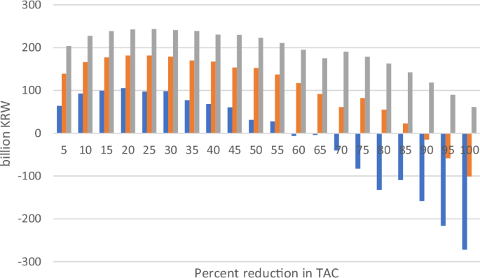
Present discounted value of the change in rent, value-added, and aggregate welfare from TAC reductions.

Full size image

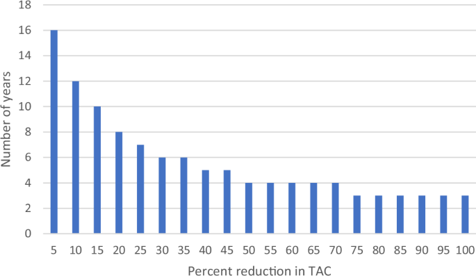
Figures 4 and 5 present the results from the baseline simulation (Also see Table 2). Figure 4 presents the changes in the mackerel sector’s rent, its value-added, and aggregate welfare (all in SSPDV over the 30 years) obtained from the 20 different scenarios. Figure 5 illustrates the number of years it takes for the level of stock to reach the target biomass level under the 20 scenarios. Results indicate that as the size of the TAC cut becomes larger (or equivalently, the rapidity of stock recovery increases), the effects of stock rebuilding on the value-added and the aggregate welfare become larger up to a certain level of TAC reduction. However, there is a tradeoff between the rapidity and the effects beyond that level.

Number of years taken to achieve the target biomass.

Full size image

The increase in the mackerel sector’s value-added is the largest when the TAC is cut by 35% (Fig. 4), with the number of years required to achieve the target biomass level being 6 years (Fig. 5). In comparison, the aggregate welfare gain is the largest when the TAC is cut by 20% with the number of years being 8 years. It takes 16 years for the stock to achieve Bmsy if the TAC is cut by only 5%, while it takes only 3 years if TAC is cut by over 75% (Fig. 5). Compared to these two measures (the mackerel sector’s value-added and the aggregate welfare), the rent increase fluctuates across the 20 scenarios (Fig. 4). The magnitude of the effects on rent depends on the relative strength of several different variables including fish price, harvest, the cost of harvesting, and effort. Figure 4 demonstrates that the rent increases by the largest amount when the TAC is cut by 70%.

We now present the results from the sensitivity analyses for three parameters: the intrinsic growth rate, the initial ratio of biomass to carrying capacity, and the discount rate because the sensitivity analyses for these three parameters provide more meaningful results than those for the other parameters (Figs. 6–8, Table 2). Since the results from the sensitivity analysis for the elasticity of substitution in production are not shown to be very sensitive, we do not report them, although they are available upon request. The results from the sensitivity analyses for all the other parameters are presented in Supplementary Information, Section D. Table 2 summarizes the results from all simulations, including the baseline simulation and all the sensitivity analyses discussed in this section and Supplementary Information, Section D.

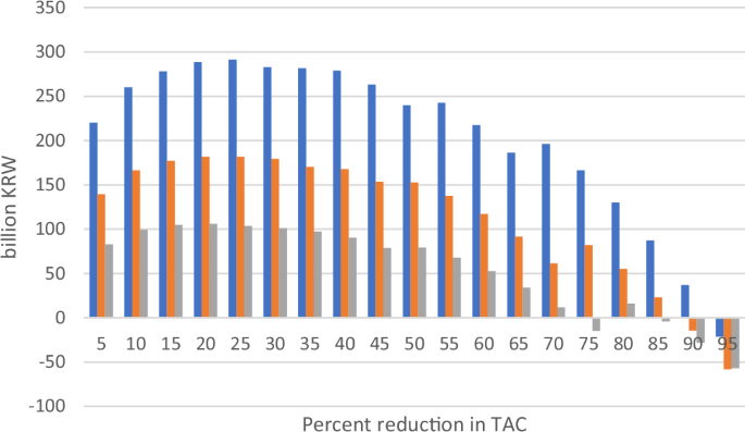
Change in aggregate welfare with different growth rates.

Full size image

Change in aggregate welfare with different ratios of biomass to carrying capacity.

Full size image

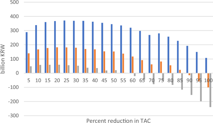
Change in aggregate welfare with different discount rates.

Full size image

A previous study estimated the intrinsic growth rate of mackerel to be 0.42, with lower and upper bounds being 0.27 and 0.66, respectively²⁰. In the baseline simulation, we used 0.42. For the present sensitivity analysis, we use the lower and upper bounds. From this sensitivity analysis, we found that the amount of time needed to rebuild the biomass depends critically on the growth rate, especially when the percentage reductions in the TAC are relatively small. In the case where the TAC is cut by 5%, it takes 25 years to rebuild the stock if the growth rate is small (0.27), while it takes only 11 years with a large growth rate (0.66) (not shown).

We also found that, under all three criteria, the amount of time to rebuild the stock varies significantly depending on the growth rates (Table 2). For instance, with the low growth rate, it takes 7 years to rebuild the stock for the rent to increase by the largest amount, while it takes only 3 years with the high growth rate (Table 2). Figure 6 illustrates that the larger the growth rate, the larger the welfare gain under each of the 20 TAC reduction scenarios. It also illustrates that the rebuilding plan can result in a deterioration of the aggregate welfare if the TAC is reduced too drastically in the early years (by more than 70%) when the growth rate is low.

In the baseline simulation, the initial ratio of the biomass to the carrying capacity is 0.291. For a sensitivity analysis, we set the ratio at 0.233 and 0.350 which are, respectively, 20% lower and 20% higher than the value used in the baseline simulation. This sensitivity analysis reveals that the size of the percentage reduction in TAC that yields the largest rent increase decreases from 70% to 50% when the initial ratio drops from the baseline level (0.291) to the low level (0.233) with the number of years increasing from 4 to 6 years (Table 2).

Results also indicate that the larger the initial level of the biomass relative to the carrying capacity, the smaller the increase in the aggregate welfare (Fig. 7). In general, the smaller (larger) the ratio of biomass to carrying capacity, the longer (shorter) it takes to reach the target biomass with all three measures of the rebuilding benefits (Table 2). This is not an unexpected result because, with a higher initial ratio of biomass to carrying capacity, the size of the increase in the biomass needed to reach the target level will be smaller, meaning that the aggregate welfare gain will be smaller. It is notable, however, that the results in Fig. 7 are very sensitive to the initial ratio.

In the baseline simulation, we used a discount rate of 4.5%²². We increase this value to 10% and then lower it to 1% for a sensitivity analysis. As the discount rate increases from the baseline level (4.5%) to 10%, the size of the percentage reduction in the TAC yielding the largest rent gain decreases from 70% to 45% (Table 2), with the number of years needed increasing by only one year (from 4 to 5 years). As the discount rate decreases from the baseline level to 1%, the size of the percentage reduction in the TAC yielding the largest gain in the aggregate welfare increases from 20% to 25% (Table 2), with the number of years needed decreasing from 8 to 7 years. The analysis reveals that aggregate welfare can deteriorate if the government reduces the TAC by over 60% when the discount rate is high (Fig. 8).

Table 2 summarizes the results obtained from all the simulations in our study (the baseline simulation and all the sensitivity analyses, including those in Supplementary Information, Section D). Results in the table indicate that the percentage reduction in the TAC yielding the largest rent increase ranges from 45% to 70%. In this case, it takes 3–7 years (mostly 4 years) to rebuild the stock. The percentage reductions in the TAC required to produce the largest value-added gain are 30–45%, with the corresponding number of years taken ranging from 4 to 9 years (mostly 6 years). In comparison, the TAC reductions that result in the largest aggregate welfare gain are 20–35%, with the number of years ranging from 5 to 12 years (mostly 8 years).

Previous studies relied on a partial equilibrium approach to examining the economic effects of fish stock rebuilding. While these studies provide useful insights, they are subject to the weakness that the effects on non-fishing industries are ignored. Our CGE model overcomes this weakness. We found from the baseline simulation that up to a certain level of the TAC reduction, the aggregate welfare gain becomes larger as the size of the TAC reduction becomes larger or as the rapidity of stock recovery increases. Beyond that level, however, there is a tradeoff between the rapidity and welfare gain; that is, a tradeoff between the ecological benefits and the economic benefits. A similar result is obtained for the mackerel sector’s value-added, the only difference being the magnitude of the TAC reduction and the number of years taken.

Sensitivity analyses for the intrinsic growth rate and the initial biomass relative to the carrying capacity elucidate the importance of accurately estimating these parameters because they affect the results in a significant way. Additionally, results are also shown to be sensitive to the discount rate. We found that a higher discount rate leads to a decrease in the size of the percentage reduction in the TAC, which yields the largest increase in the mackerel sector’s rent and its value-added (Table 2). Choosing the discount rate depends on the preferences of the mackerel fishermen for the future benefits from rebuilding the stock (or the preferences of the regional residents as a whole for the aggregate welfare). A low discount rate means that the mackerel fishermen are relatively sure that they will receive the future benefits from stock rebuilding because they trust the fishery manager’s rebuilding policy or because they are given a promise of receiving the future benefits via a rights-based management system such as an individual transferable quota (ITQ) system. On the other hand, a high discount rate reflects the uncertainty about the future benefits of the stock rebuilding. In this case, to the mackerel fishermen, future benefits count for relatively little. In the extreme case that the benefits count for nothing, they may have an incentive to treat the fish stock as a non-renewable resource to be mined^23,24.

The results in Table 2 might shed some light on the government policy for stock rebuilding. Fishery managers/regional policymakers are faced with the question of which criterion they have to use when deciding between fish stock rebuilding options (scenarios)—the rent of the fishing sector at hand (here, the mackerel sector), its value-added, or the aggregate regional welfare. If their primary concern is the fishermen’s rent (as many studies relying on the partial equilibrium approach often implicitly assume), they may choose to reduce the TAC rather significantly—by 45–70%. In this case, it will take a relatively short amount of time to rebuild the stock; that is, 3–7 years (mostly 4 years). If, instead, they care more about the mackerel sector’s value-added, they may choose to reduce the TAC by less (30–45%), which will take slightly more time (4–9 years, mostly 6 years). On the other hand, they may be more concerned with the benefits of stock rebuilding to the society as a whole, including not only the benefits to the fishermen but also those accruing to other sectors of the economy^25,26,27,28. In this case, they may choose the option that reduces the TAC by a much smaller percentage (20–35%) with many more periods (5–12 years, mostly 8 years) required to recover the stock because this option yields the largest aggregate welfare gain, which is a measure of the total societal benefits.

Suppose the government chooses the option that yields the largest rent to the fishermen. As results from our study indicate, this option will entail a large reduction in the TAC in the early periods. This will have negative effects on other sectors of the economy because it means (i) a reduction in non-fish inputs used for fish harvesting, (ii) a subsequent decrease in the production by the industries that supply the non-fish inputs, and therefore, (iii) a deterioration of the overall welfare of the residents of the region. Results from the baseline simulation reveal that a reduction of TAC that is larger than 20% will lead to an acceleration of the stock recovery but at the cost of the deteriorated aggregate welfare. In the extreme case where the TAC reduction is over 90%, the aggregate welfare even declines, compared to its pre-policy level due to the stock rebuilding. Furthermore, even the fishermen may hesitate to accept the first option (largest rent), although it generates the largest rent over time because this option entails a substantial decrease in their short-term income.

This implies that the government may want to avoid some extreme options, such as the TAC reductions that are too small or too large. If the government attempts to recover the biomass too rapidly by a significant reduction in the TAC, it may deteriorate the aggregate welfare and face some resistance from the fishermen who want to eschew the short-term loss in their income. On the other hand, if the reduction in the TAC is too small (e.g., 5%), it will take a longer time than expected to recover the stock while not yielding the largest increase in any of the three measures of the benefits (rent, value-added, and aggregate welfare). Currently, the Korean government sets a maximum of 15 years as the time limit for rebuilding a fish stock. This study suggests that it is feasible to rebuild the stock within this time frame (15 years) unless the intrinsic growth rate is low (0.27), the initial ratio of biomass to the carrying capacity is small (0.233), and the annual reduction in the TAC is too small (<5%).

In this section, we present a brief description of the Busan CGE model. Supplementary Information, Section A, provides more details about the model while Supplementary Information, Section B, presents a full list of equations, parameters, and variables used in the model.

The Busan CGE model has 36 industries (sectors) and 36 commodities, each of which is produced by the corresponding industry (Supplementary Information, Section C, Supplementary Table C.1). The industries include two wild fish harvesting industries [mackerel harvesting industry (sector) and non-mackerel harvesting industry (sector)], one aquaculture industry, one fish processing industry, and 32 non-seafood industries.

Production in each fish harvesting sector is determined through a three-stage optimization process (Fig. 9). In the first stage, harvest (H) is determined by a Cobb–Douglas (CD) aggregation of fishing effort (E) and fish biomass (N):

where F(E, N) is the harvest function, d is the shift parameter (or catchability parameter), and f and g are, respectively, the effort and stock elasticities.

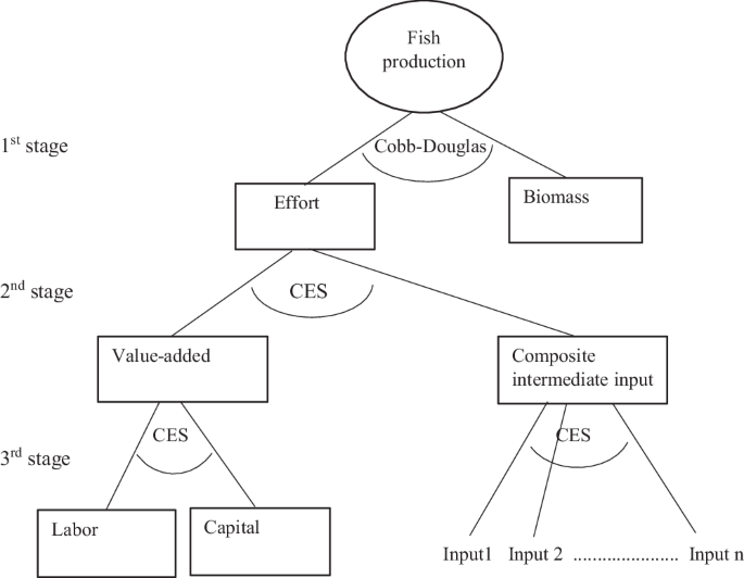
Nested fish production function.

Full size image

Maximizing profit subject to the harvest function and the TAC level where the fishermen exhaust the full TAC, the effort demand function is derived as

where PVI is the price (cost) of value added plus intermediate inputs used to produce one unit of output, net of indirect business taxes (i.e., the price of one unit of output minus indirect business taxes); (eta) is the marginal surplus of producing another unit of output; and C is the unit cost of effort with the effort being a combination of labor, capital, and intermediate inputs. Here, (({{rm {PVI}}}-eta )) is the virtual price²⁹ of the constrained output; that is, the price of output (net of indirect business taxes) that would induce the firm to choose H = TAC.

In the second stage, the value-added composite (LAK) and the composite intermediate input (INT) are combined to produce effort via a constant returns to scale (CRS), constant elasticity of substitution (CES) function. Cost minimization subject to the effort function yields demands for LAK and INT. In the third stage, firms combine labor (L) and capital (K) according to a CES value-added function to obtain the valued-added composite (LAK) and combine individual intermediate inputs according to another CES function to form the composite intermediate input (INT). In a similar way to the second stage, the third stage yields demand functions for labor, capital, and individual intermediate inputs, along with the associated unit cost functions.

The production structure of the non-fishing industries is similar to that of the fish harvesting industries, except that there are no effort or biomass variables in their production. Firms in the non-fishing industries combine the composite value-added and the composite intermediate input using a CES function in the first stage. The optimization process in the second stage is the same as that for the third stage in fish harvesting industries’ production.

Our model has one aggregate representative household. We use a multi-level nested CES utility function to represent the preference of the household in the region, which allows flexibility in assigning different values of the elasticity of substitution for different (groups of) commodities (including fish) (Fig. 10). To determine the quantities of the commodities consumed by the regional household, we use a four-stage optimization procedure. In the first stage, the demands for the composite food commodity (FD) and the composite non-food commodity (NFD) are determined by maximizing the utility represented by the CES function subject to its budget constraint, yielding the demand functions for FD and NFD.

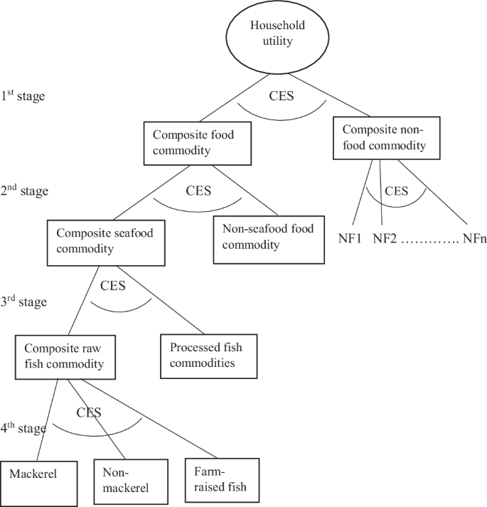
Nested utility function.

Full size image

In the second stage, given the quantity of FD in the first stage, the demand functions for the composite seafood commodity and the composite non-seafood food commodity are derived by minimizing the cost of these two composite goods subject to a CES FD aggregation function. Similarly, in this stage, the demands for the individual non-food commodities (NF1, NF2, …, NFn) are determined by minimizing the cost of these commodities subject to a CES NFD aggregation function. We follow a similar procedure to derive the demands for the composite raw fish commodity and processed seafood in the third stage. Finally, in the fourth stage, the demands for the individual raw fish commodities (i.e., mackerel, non-mackerel, and farm-raised fish) are derived. By specifying several different nests in the household preference, as shown in Fig. 10, we can assign different elasticities of substitution in the different nests.

Users of a commodity (households, industries, and government) in Busan consume a combination of three different versions of the commodity sourced from three different places—the study region, the rest of the country (ROC), and foreign countries. We assume that the three different versions are qualitatively different and imperfect substitutes for each other and that their prices can be different³⁰. The users undertake a three-stage optimization to determine their consumption of the commodity (Fig. 11). In the first stage, the region’s total demand for each commodity is determined by adding up the demands from households, industries (intermediate demand, investment demand), and governments.

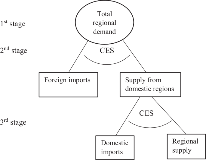
Nested Armington function.

Full size image

Once the total demand is determined in the first stage, the second stage computes the quantities of the commodity sourced from the country and its imported counterpart from foreign countries by minimizing their expenditure on the two different versions of the commodity subject to a CES Armington function³⁰. This yields an import demand function for the foreign-sourced commodity (M), which is downward sloping.

Given the composite commodity sourced from domestic regions in the second stage (D), the third stage determines the quantities of regionally produced commodity and the version sourced from ROC by minimizing the total expenditure on the two different versions of the commodity subject to another CES Armington function. This yields the import demand function for the commodity from ROC, which is also downward sloping.

For foreign imports, this study adopts the “small country (region)” assumption that the region’s imports of goods (including fish) from foreign countries do not wield a strong power in the foreign markets. This means that the region faces an infinitely elastic import supply function for foreign-sourced goods and that the prices of imports from foreign countries are fixed at their base-year levels. On the other hand, since Busan is one of the major economic regions within Korea greatly influencing the pricing of the commodities in domestic markets through domestic imports, the region is assumed to face an upward-sloping import supply curve (i.e., less-than-infinite elasticity) for the goods imported from ROC.

Firms in Busan undertake a three-stage optimization to distribute their output (Fig. 12). In the first stage, they determine their output level by maximizing profit (or minimizing cost). Once the total output of a commodity is determined in the first stage, they determine in the second stage the quantities of the commodity supplied to two different destinations—domestic regions (including the study region) and foreign countries, by maximizing their revenues from sales of the commodity to the two different markets subject to a constant elasticity of transformation (CET) function. This yields an export supply function for the commodity exported from the region to the foreign market, which is upward-sloping.

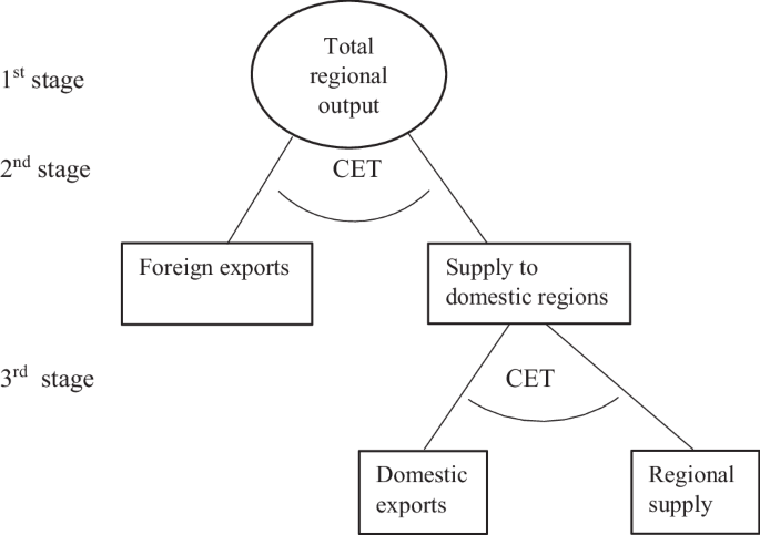
Nested CET function.

Full size image

In the third stage, given the quantity of the composite commodity supplied to domestic regions (G) from the second stage, the firms maximize their revenue from sales of the commodity to two different domestic regions (the study region and ROC) subject to another CET function. This yields an export supply function for the commodity exported to ROC. Again, this study adopts the “small country (region)” assumption that the region’s exports of goods (including fish) to foreign countries do not substantially influence the pricing of the goods in foreign markets. This means that the region faces an infinitely elastic export demand (i.e., foreign countries’ demand) for the goods from the region and that the price of the exports to the foreign countries is fixed at its base-year level. As in domestic imports above, it is assumed that the region exercises strong power in ROC’s market via its exports and that the region faces the export demand (i.e., ROC’s demand) for the goods produced in the region that is less than infinitely elastic.

Supplementary Information, Section C (Supplementary Table C.2) provides further descriptions of the domestic and foreign trade-related functions and the values of the elasticities used in the baseline simulation. The elasticity values in Supplementary Table C.2 are from Supplementary Table C.3 (Supplementary Information, Section C).

Several CGE studies of fisheries assume that the total stocks of labor and capital (vessels) available in the study region are fixed^31,32. This means that if the fishing industry frees up some of the factors of production due to a policy change (e.g., a lower TAC), they can flow to non-fishing industries within the region. Another CGE study assumes that capital is fixed in the rationalized sector both before and after the fishery reform as well as in each of the non-fishing industries¹⁵.

The factor mobility assumptions used in these studies may be appropriate for their respective study regions. Furthermore, there is no strong empirical evidence regarding the inter-sectoral and inter-regional mobility of factors used in fisheries. In the present study, the labor released from the mackerel sector due to a lowered TAC may or may not remain in the region. Thus, this study first assumes that total labor in the region is fixed and, therefore, that the labor discharged from the mackerel sector stays and finds employment elsewhere in the region with the market wage rate endogenously determined (baseline simulation). Later, our study relaxes this assumption in sensitivity analysis and assumes that labor is mobile between the region and ROC, meaning that the market wage rate is fixed and equalized between the regions.

For most fisheries, including Busan’s mackerel fishery, if capital is freed up by a fishery due to a government policy (reduction in TAC in our study), it will either exit (disappear from) the study region (non-malleable capital) or stay within the region and be reinvested in non-fishing sectors (malleable capital). Therefore, this study assumes in the baseline simulation that the fishing capital from the mackerel sector exits the region with the return to capital fixed and equalized between the study region and ROC (perfect capital mobility assumption). Later, a sensitivity analysis is performed to examine how the results vary if capital is assumed to stay within the region, finding employment in the non-seafood industries. A previous study discusses additional possibilities of inter-sectoral and inter-regional factor mobility for fisheries³³.

When the harvest level (HARV) changes due to stock rebuilding, it changes the stock level (N). In this study, we assume that stock grows following the logistic growth function:

where N_t is the stock level in period (year) t, γ is the intrinsic growth rate, KC is the carrying capacity, and HARV_t is the harvest level (in tons) in period t. Thus, the increase in the stock level will raise the marginal productivity of effort via Eq. (1). Note that the harvest level (H) in Eq. (1) measures the fish production calibrated with its base-year price set to one. HARV in Eq. (3) measures the fish production in its actual weight (tons).

The Busan social accounting matrix (SAM) is used to develop the Busan CGE model. Descriptions of the parametrization and calibration are presented in Supplementary Information, Section C. To develop the Busan SAM, this study uses 16-region, 33-sector multi-regional input-output (MRIO) data for 2015³⁴. Busan is one of the 16 regions. This MRIO dataset provides for each of the 16 regions the information on (i) inter-industry transactions within the region, (ii) employee compensation, (iii) operations surplus, (iv) indirect business taxes, (v) final demand (consumer demand, investment demand, government demand, and both domestic and foreign exports) for commodities, (vi) the transactions between each of the industries in the region and each of the industries in the other regions, and (v) imports from, and exports to, other domestic regions and foreign countries. All 15 non-Busan regions are integrated into the rest of the country (ROC). Next, the trade flows between Busan and ROC and those between Busan and the rest of the world (ROW) are separately estimated based on the MRIO data.

To estimate the total government demand, we first combine government expenditure with government investment for each commodity in the Busan IO data. Next, the single government sector in the data is divided into two government sectors, the national government and the regional government. In our study, the regional government is the combination of the provincial government (i.e., Busan government) and all the lower-level governments (e.g., Kus and Dongs). Information on regional government expenditures is from the Local Finance Integrated Open System (LFIOS)³⁵. To obtain the national government demand, we subtract from the total government demand the regional government expenditures. The national government revenues (taxes) and expenditures on items other than goods and services purchased by the government (e.g., transfer payments) are estimated using the National Tax Service Annual Report (NTSAR)³⁶. Regional government revenue and expenditure information are from the Annual Local Tax Statistics Report (ALTSR)³⁷ and LFIOS³⁵, respectively.

The 33-sector MRIO dataset has highly aggregated sectors and does not separately identify the fish-producing and fish-processing industries. In the dataset, fish production is included in the Agriculture, Forestry, and Seafood Production sector, and seafood processing is included in the Food and Drinking sector. Fish production is separated from the Agriculture, Forestry, and Seafood Production sector¹⁹. Then, this fish production sector is further disaggregated into mackerel production, non-mackerel production, and aquaculture¹⁹. Next, seafood processing is separated from the Food and Drinking sector. Finally, the last two industries (Other Service and Other) in the MRIO dataset are combined into a single sector. Thus, the number of industries in the final SAM is 36 (Supplementary Information, Section C, Supplementary Table C.1). Data on household tax payments to the national and regional governments are from the Household Income and Expenditure Survey (HIES)³⁸, NTSAR³⁶, and ALTSR³⁷.

Using the data thus estimated as above, Busan SAM is constructed and is available upon request. When balancing the SAM, we adjust the elements in the exogenous accounts until the column sums equal the row sums. This study uses this method to balance the SAM rather than using bi-proportional adjustment techniques (e.g., RAS technique) in order to keep the original parameter values (e.g., production functions and other key behavioral and endogenous share parameters) implied in the SAM, but allow the peripheral elements in the exogenous accounts to be adjusted when necessary to balance row and column totals.