Efficiency of neural quantum states in light of the quantum geometric tensor

Recent years have seen immense growth in the use of machine learning (ML) methods in the field of quantum many-body physics. Central to this intersection are Neural Quantum States (NQSs), which are currently revolutionizing Variational Monte Carlo (VMC) approaches and related applications^{1,2,3,4,5,6,7,8}. Their success relies on the expressivity of neural networks (NNs), which have the theoretical capacity to represent any state, with a large enough number of parameters. This is formalized by so-called (i) universal representation theorems, asserting that the approximation error inherent in an NN (and by extension, in an NQS) can approach zero asymptotically as one increases the network’s width or depth, contingent on locating the global minimum of the loss function^9,10,11,12. Additionally, it is well-understood in the standard ML context that (ii) increasing the number of parameters beyond the over-parameterization limit leads to a smoother loss landscape and faster convergence^13,14.

Building on those principles, numerous variational studies have increased the width or depth of NNs in order to check convergence in calculations where the ground state is found by energy minimization^1,15,16,17. A striking example can be found in Fig. 2 of ref. ¹⁷, where the NQS approximation error at convergence systematically decreases as the number of parameters of a ResNet increases, ultimately reaching numerical precision at the largest parameter size. This approach is quite general and is also employed when simulating the real-time dynamics¹⁸, and the steady-state in open quantum systems^5,19.

However, exceptions to this rule do emerge in practical calculations, i.e., instances in which an NQS fails to become more accurate as the number of parameters increases. We will call this situation a practical limitation to reach universal representability. We stress that this is not in opposition to the representation theorems, which are valid only when the global minimum can be found, in the limit of a sufficiently large number of parameters. A practical limitation to reach universal representability with a specific minimization algorithm might occur because the additional parameters cannot be used effectively even after the minimization has converged. As a result, the global minimum cannot be found with a reasonable computational budget.

Moreover, it is unclear what the additional parameters encode once the optimization has converged. Several results in standard ML tasks^20,21,22, and Variational Quantum Algorithms²³ document the existence of redundant directions in the parameter space, suggesting that the encodings are locally highly degenerate. This is in clear opposition to tensor networks and matrix product states (MPSs) in particular, where increasing the bond dimension is linked with the increase in the maximal entanglement entropy of the state^24,25. Instead, while it has been shown that even simple NQSs can encode states with arbitrary entanglement^26,27,28, we do not know what states NQSs with a finite number of parameters cannot encode. The role of parameters in an NQS and their relationship to the overall accuracy of a calculation is therefore unclear. While in some cases, it is possible to invoke some theorems as an explanation for the effectiveness of increasing the number of parameters, we still do not understand what happens in the presence of a practical limitation to reach universal representability.

Nevertheless, it is possible to quantify the role of parameters in an NQS by looking at the Quantum Geometric Tensor (QGT), which is a generalization of the Fisher Information Matrix (FIM) in the context of variational wavefunctions^29,30. In addition to its usage in the stochastic reconfiguration (SR) method^31,32, a few studies have used the QGT to identify the relevant parameters in a variational optimization^33,34.

In this work, we investigate the practical representation ability of a restricted Boltzmann Machine (RBM) as an NQS ansatz in a simple setting: the search for the ground state of a one-dimensional quantum spin model. We chose the spin-1 bilinear-biquadratic (BLBQ) chain because of its diverse phase diagram encompassing the topologically ordered gapped Haldane phase and the gapless extended critical phase. This makes it an ideal test bed for our study. To directly investigate the representation ability of the NQS ansatz, we choose to employ a supervised learning procedure with the NQS to represent a given ground state, i.e., we optimize the infidelity of the NQS ansatz w.r.t. the exact ground state. We perform infidelity optimizations at various network densities of the NQS ansatz to study the impact of network density on the NQS ground state approximation. We use an NQS ansatz given by a modified RBM (see Methods section) suitable for spin-1 systems¹⁵. We optimize the infidelity using the natural gradient descent (NGD) algorithm, which is essentially a generalized version of the SR method³², applicable to any supervised learning procedure. The gradients and the QGT matrix are computed exactly to exclude biases induced from sampling in the Monte Carlo procedure.

To analyze our results, we propose a notion of the dimension of the relevant manifold d_r of a variational ansatz, given by the rank of the QGT (described in detail in the subsection “Quantum Geometric Tensor” in the Results section). Furthermore, we also identify a strict upper bound for the rank of the QGT, which we call the effective quantum dimension d_q, given the task of representing the ground state of a particular Hamiltonian. We establish that the ratio d_r/d_q can be used as a local probe to understand the evolution of the NQS approximation with the size of the network, as well as the case of a practical limitation to reach universal representability. Furthermore, we demonstrate that d_r/d_q is an important indicator for characterizing the efficiency of an NQS ansatz in representing a given ground state as the network width increases.

BLBQ spin-1 chain

The spin-1 BLBQ model in one dimension is defined by the Hamiltonian:

More generally, the Hamiltonian is written as (H={sum}_{i}J[cos (theta ){{{{bf{S}}}}}_{i}cdot {{{{bf{S}}}}}_{i+1}+sin (theta ){({{{{bf{S}}}}}_{i}cdot {{{{bf{S}}}}}_{i+1})}^{2}]) in the literature^35,36. The model is parametrized by an angular variable θ, and ({{{{bf{S}}}}}_{i}=({S}_{i}^{x},{S}_{i}^{y},{S}_{i}^{z})) is the spin operator acting on the local spin-1 Hilbert space at site i. The above Hamiltonian has a gapped Haldane phase^37,38 for  −π/4 < θ < π/4, an extended critical phase^{35,39,40,41,42} for π/4 ≤ θ < π/2, a ferromagnetic phase for π/2 ≤ θ < 5π/4, and a dimerized phase for  −3π/4 < θ < −π/4^36,43 (Fig. 1). We focus on the Haldane phase and the extended critical phase in this work. The Haldane phase describes the isotropic Heisenberg antiferromagnet at θ = 0. It is characterized by a hidden topological order, which is the strongest for the Affleck-Kennedy-Lieb-Tasaki (AKLT) state^44,47,46 at (theta =arctan (1/3)). The AKLT state is a valence-bond state, which can be represented by two spin-1/2 particles at each site, forming singlets with the spins of the neighboring sites (see supplementary Note 1). The AKLT state has an exact MPS representation with bond dimension 2⁴⁷. It is also the state that has the lowest bipartite entanglement in comparison to ground states at other values of θ⁴⁸. The Haldane phase is gapped and has a ground state with an exponentially decaying antiferromagnetic spin-spin correlation in the thermodynamic limit. Up to the AKLT point, the correlation function behaves as (langle {S}_{0}^{alpha }cdot {S}_{j}^{alpha }rangle approx {(-1)}^{j}exp (-j/xi )/sqrt{j}) with a correlation length (xi =1/ln (3)) for the AKLT state. For (arctan (1/3) < theta < pi /4), the modulation wavevector shifts away from k = π to reach k = 2π/3 at θ = π/4. The Haldane gap closes at θ = π/4, marking a critical point, known as the Uimin-Lai-Sutherland (ULS) point^41,42,49, across a Berezinskii-Kosterlitz-Thouless (BKT) transition^35,50. At this point, the model has an exact SU(3) symmetry and is integrable. Its low-energy physics is described by the Wess-Zumino-Witten (SU(3)_k = 1) conformal field theory^35,45,50. The model remains gapless in the thermodynamic limit throughout the region π/4 ≤ θ < π/2. In this phase, the dominant correlations are of quadrupolar nature, with wavevector k = ± 2π/3, and decay as a power law with exponent η = 4/3^35,39.

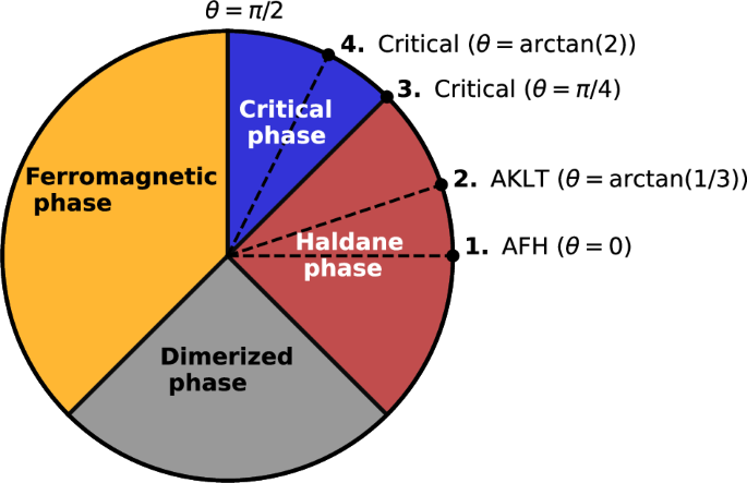
We perform infidelity (Eq. (2)) minimization, with a neural quantum state (NQS) ansatz given by a modified restricted Boltzmann machine (RBM) for spin-1 models¹⁵ (described in Methods section), at the four marked points in the phase diagram: antiferromagnetic-Heisenberg (AFH), Affleck-Kennedy-Lieb-Tasaki (AKLT), and the two critical phases at θ = π/4, and (arctan (2)) respectively.

Full size image

Minimizing the NQS infidelity

We search for NQS approximations of the ground states in the Haldane and the critical phases of the spin-1 BLBQ chain by minimizing the infidelity of the NQS w.r.t. the exact ground state (| Omega left.rightrangle) (see Methods section for more details),

Here (| {psi }_{theta }left.rightrangle ={sum}_{n}{psi }_{theta }(n)| nleft.rightrangle) is the NQS and (| nleft.rightrangle) denotes a state in the computational basis. Note that the degree to which the NQS ansatz represents the true ground state is given by the fidelity f = 1 − I ∈ [0, 1], and hence, the infidelity I gives the error in the NQS approximation for the ground state. For comparisons, we also perform the usual VMC procedure, included in the supplementary Note 2, where one minimizes the energy

to get an NQS approximation for the ground state. Here ({p}_{theta }(n)={leftvert {psi }_{theta }(n)rightvert }^{2}/leftlangle right.{psi }_{theta }| {psi }_{theta }left.rightrangle) is the probability distribution over the computational basis. For the rest of the paper, we focus on the results of the infidelity minimization procedure. We restrict our computations to the total S_z = 0 sector of the Hilbert space.

We report the infidelities at convergence of the infidelity minimization with NGD in Fig. 2, for different sizes of the BLBQ chain L = 8, 10, 12, for four phases in the phase diagram (the four points marked in Fig. 1), and for different hidden layer densities α. As we increase α, the converged infidelities for the different phases reduce to very low values and saturate thereafter at a certain value of α in most cases for L= 8, 10. The converged infidelities for the four phases for L = 12 oscillate after an initial descent as α increases. We also remark that the NQS for the AKLT state has the best approximation (the minimum infidelity) in most cases. This is consistent with the fact that the AKLT state has the lowest entanglement (has an exact MPS representation with bond dimension 2), among all the other phases.

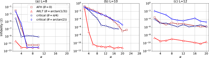
Infidelity (I) after the convergence of an exact infidelity minimization procedure is shown as a function of α, for the antiferromagnetic-Heisenberg (AFH) (red squares), Affleck-Kennedy-Lieb-Tasaki (AKLT) (red triangles) and the critical phases (blue circles and blue diamonds for θ = π/4 and (arctan (2)) respectively) of the spin-1 BLBQ chain with open boundary conditions. Results are shown for chain lengths a L = 8, b L = 10, and c L = 12. The neural quantum state (NQS) used is a modified restricted Boltzmann machine (RBM) for spin-1 systems¹⁵ (see Methods section).

Full size image

To avoid artefacts originating from the Monte Carlo sampling⁵¹ and solely investigate the representation power of the NQS ansatz, we perform the infidelity minimization by summing over the total S_z = 0 subspace of the Hilbert space.

Additionally, we check that the infidelity minimization has converged well by inspecting the local infidelity landscape through the Hessian (see supplementary note 5 for the spectra of the Hessian for L = 8). Our solutions lie in a deep valley (many large positive eigenvalues), which has a few infinitesimally small downward slopes (few very small negative eigenvalues) as commonly seen in the ML literature^52,53.

A systematic decrease in the NQS approximation error with α to numerical precision, followed by a saturation, is consistent with our expectations from the universal representation theorems. This is the case for infidelity optimizations for the AFH, AKLT, and the critical phase at (theta =arctan (2)) with L = 8, as well as for the AKLT phase with L = 10, where we achieve converged infidelities ≤ 10⁻¹¹. For practical purposes, we consider having reached numerical precision in the above cases. For the other cases, the infidelities either saturate at a larger value with small oscillations, which we call a premature saturation of the infidelity, or continue to decrease with α. The latter could suggest that the NQS needs more parameters to be able to approximate the solution better. However, a premature saturation of the infidelity suggests that the optimized NQS is locally not able to use the newly added parameters to improve the solution. This scenario can be further investigated by examining the Fubini-Study (FS) metric in the space of variational wavefunctions. From this metric, we derive the QGT^29,30, which gives a measure of the relevant directions in the parameter space, as discussed in the following paragraphs.

Quantum geometric tensor

In defining a distance measure between two pure states, one must consider that states differing by a global phase are physically indistinguishable⁵⁴. Consequently, the set of pure states is isomorphic to the set of rays in the Hilbert space, i.e., to the projective Hilbert space, over which a metric can be unambiguously defined^55,56. The FS metric naturally emerges as the unique (up to a constant factor) Riemannian metric on the set of rays, being invariant under all unitary transformations, that is, under all possible time evolutions⁵⁷. For two pure states (| {psi }_{theta }left.rightrangle) and (| {psi }_{phi }left.rightrangle), parameterized by θ and ϕ, the FS distance is defined as:

For an infinitesimal variation ϕ = θ + dθ, a second-order expansion of the squared FS distance yields the line element:

where the QGT

captures the local curvature of the space. Note that the above expression holds for the case when the variational state (| {psi }_{theta }left.rightrangle) is normalized. In the general case, the QGT takes the form ({{{{{rm{G}}}}}}_{ij} = frac{leftlangleright.{frac{partial psi_{theta}}{partial theta_{i}}}|{frac{partial psi_{theta}}{partial theta_{j}}}left.rightrangle}{leftlangleright.{psi_{theta}}|{psi_{theta}}left.rightrangle} – frac{leftlangleright.{frac{partial psi_{theta}}{partial theta_{i}}}|{psi_{theta}}left.rightrangleleftlangleright.{psi_{theta}}|{frac{partial psi_{theta}}{partial theta_{j}}}left.rightrangle}{{leftlangleright.{psi_{theta}}|{psi_{theta}}left.rightrangle}^2}). The QGT matrix is positive semi-definite, ensuring that its eigenvalues are real and non-negative. These eigenvalues measure the curvature of the FS distance along the associated eigendirections. Non-zero eigenvalues correspond to relevant directions where the quantum state undergoes significant variation, while zero eigenvalues indicate redundant directions where parameter changes produce no meaningful change in the quantum state³⁰. Thus, at convergence, the rank of the QGT reflects the number of relevant directions (d_r), or the dimension of the relevant manifold, that the variational ansatz uses to represent the quantum state. In the special case where wavefunction amplitudes are real and positive, that is (| {psi }_{theta }left.rightrangle ={sum}_{n}sqrt{{p}_{theta }(n)}| nleft.rightrangle), the QGT simplifies to a scaled version of the classical FIM²⁹. Specifically,

where the averages are taken with respect to the Born probability distribution p_θ(n) over the states (| nleft.rightrangle). ({{{mathcal{F}}}}) is the FIM of the probability distribution p_θ(n) and arises from the second-order expansion of the Kullback-Leibler divergence, a proximity measure between probability distributions.

Natural gradient descent

Standard gradient descent (GD) algorithms attempt to minimize the loss function iteratively by moving in the direction of steepest descent under Euclidean geometry. This is done following the prescription

where δθ is the parameter update, η is the learning rate, and F is the conjugate gradient of the loss function in Eq. (2) (see Methods section). As a result of assuming an underlying Euclidean geometry, GD is poorly suited to navigate the projective Hilbert space due to the geometry of the space itself, and the parameter redundancy introduced by an NN parametrization⁵⁴. Thus standard GD often struggles in landscapes with steep valleys or flat plateaus where convergence can be slow as updates oscillate in steep directions while taking small steps in shallow ones.

NGD improves upon this by adapting parameter updates to the intrinsic geometry of the function space, as defined by the QGT^29,58,59,60. Instead of relying on the Euclidean gradient, NGD employs the geometry-aware update rule (see supplementary Note 3):

The action of the QGT inverse G⁻¹ can be heuristically understood as locally “flattening” the landscape. NGD offers several key advantages. First, by adjusting for local curvature, NGD prevents overshooting in steep directions and accelerates progress in flat regions. Furthermore, NGD is first-order invariant under reparameterization, ensuring consistent optimization across different representations. Ultimately, NGD is less prone to slow convergence near saddle points or local minima guaranteeing faster convergence under a variety of conditions^61,62.

Effective quantum dimension

One can express Eq. (6) as

where ({hat{O}}_{mu }={sum}_{n}partial /partial {theta }_{mu }| nleft.rightrangle leftlangle right.n|) is a partial derivative operator, and (| nleft.rightrangle) is a state in the computational basis. Eq. (10) can then be represented as a matrix multiplication ({sum}_{n}{M}_{alpha n}^{{{dagger}} }{M}_{nbeta }), where the matrix elements ({M}_{nmu }=langle n| ({hat{O}}_{mu }-langle {hat{O}}_{mu }rangle )| {psi }_{theta }rangle), and the summation over n runs over the relevant (possibly constrained by symmetries) Hilbert space. We introduce the notion of an effective quantum dimension d_q, which represents the dimension of this space. This gives the upper bound on the QGT rank d_r, given the task of representing the ground state of a specific Hamiltonian. In our case, for the spin-1 chain with the constraint total S_z = 0, and a global spin-flip symmetry, the effective quantum dimension d_q = (D + 1)/2, where D is the dimension of the total S_z = 0 subspace. Therefore, d_q = (D + 1)/2 is the maximum dimension of the relevant manifold around the optimized NQS. For our computations, d_q takes the values 554,  4477, and 36895 respectively for L = 8, 10, and 12 (for all four phases).

Rank of the QGT

We compute the QGT at convergence of the infidelity minimization procedure for each case and plot the rank of the QGT (d_r) with the hidden layer density α in Fig. 3a–c. The insets show the QGT rank normalized w.r.t. the number of parameters (N_p) in the NQS ansatz. The QGT rank d_r increases with an initial increase in α, accompanied by a decrease in the infidelity. This suggests a correlation between the accuracy of the NQS approximation and d_r. To further elucidate this correlation, we plot the converged infidelity as a function of the ratio of the QGT rank w.r.t. the effective quantum dimension, i.e., d_r/d_q, in Fig. 3d–f. This reveals that the infidelity decreases exponentially with the ratio d_r/d_q until it saturates beyond a particular value of α. For the AFH phase and the critical phase at (theta =arctan (2)), with L = 8, we achieve numerical precision at the saturation of the ratio d_r/d_q ≈ 1 (when the QGT rank takes its maximum value), i.e., when the NQS is performing at its best. While, for the AKLT phases with L = 8 and 10, we attain numerical precision even with d_r/d_q < 1, when the NQS is not yet at its full capacity. Furthermore, the NQS also performs very well for the AKLT phase with L = 12 despite a significantly lower d_r/d_q compared to the other phases. This implies that the wave function for the AKLT phase is inherently simpler to be represented by the NQS. Whereas, in cases where the infidelity saturates at higher values with some oscillations, the ratio d_r/d_q plateaus below 1. This suggests that the NQS is not able to add relevant directions around the converged solution, with an increase in α, which in turn limits its ability to improve its approximation. Note, however, that we have a small deviation from this behavior for some cases with L = 12, where the QGT rank d_r (and the ratio d_r/d_q) increases while the infidelity approaches premature saturation. This could be attributed to the decreasing normalized rank d_r/N_p in the inset of Fig. 3c, suggesting that the QGT rank increases at a slower rate than the number of parameters N_p, leading to the inability of the optimized NQS to represent the ground states with higher accuracy. This is in contrast to the case of L = 10 (for instance, for the AFH and the critical phases), where the normalized rank d_r/N_p remains constant in the regime where the optimized NQS consistently improves its approximation with an increase in α. Furthermore, it is worth highlighting that the decrease in the normalized rank d_r/N_p with α for L = 12 has a different origin than from cases (with L = 8, 10) where it occurs either due to an early saturation of d_r (i.e., when d_r < d_q) or when d_r reaches its upper bound d_q.

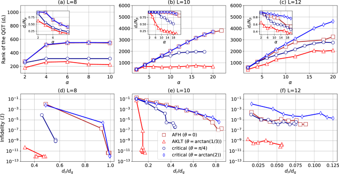
a–c The rank of the QGT (d_r) is shown as a function of the hidden layer density α for lengths L = 8, 10,  and 12. The insets show the QGT rank normalized w.r.t. the number of parameters N_p. d–f The converged infidelity (I) is shown as a function of the ratio d_r/d_q, where d_q is the upper bound for the QGT rank (or the effective quantum dimension), with d_q = 554, 4477, and 36,895, respectively, for L = 8, 10, and 12. The QGT rank d_r (which is also the dimension of the relevant manifold around the converged solution) is computed as the number of eigenvalues of the QGT greater than 10⁻⁵. Each panel shows the data for the antiferromagnetic-Heisenberg (AFH) (red squares), Affleck-Kennedy-Lieb-Tasaki (AKLT) (red triangles), and the two critical phases (blue circles and blue diamonds for θ = π/4 and (arctan (2)) respectively) of the spin-1 BLBQ chain with open boundary conditions, for a given length of the chain.

Full size image

Moreover, for a given size of the chain, the slope of the I vs. d_r/d_q plot provides a measure of the efficiency of the NQS ansatz to represent a given ground state with increasing accuracy as its width grows. For instance, for L = 10, the I vs. d_r/d_q plot has the steepest slope for the AKLT phase, suggesting that the optimized NQS ansatz represents the AKLT phase most efficiently. In contrast, the NQS ansatz represents the AFH and the critical ((theta =arctan (2))) phases with a much lower efficiency.

Spectrum of the QGT

While we demonstrated that the improvements and limitations in the NQS approximation can be analyzed using the rank of the QGT, it is also insightful to examine the spectrum of the QGT, which reveals how the local metric of the FS distance around the converged solution, evolves with α. We plot the spectrum of the QGT, for each solution with L = 10, as histograms in Fig. 4. We broadly notice two regimes in the evolution of the QGT spectra as α increases, in relation to the converged infidelities: (i) a decreasing infidelity regime (for small values of α), and (ii) a saturated infidelity regime (for relatively larger values of α). In regime (i), the QGT spectra indicate a significant increase in large-magnitude eigenvalues as α increases, resulting in an increase in the QGT rank (and the ratio d_r/d_q, indicating a growth in the dimension of the relevant manifold around the converged solution), as seen in Figs. 3 and 4. This is accompanied by a decrease in the converged infidelities. Whereas in regime (ii), the QGT spectra show an increase in very small eigenvalues as α increases, and hence the dimension of the relevant manifold (and the ratio d_r/d_q) does not change anymore. This leads to the narrow peaks at very low eigenvalues (corresponding to the redundant directions), in the histograms (Fig. 4), as can be seen clearly for the AKLT and the critical phase at θ = π/4 with L = 10. In this regime, the NQS approximation for the ground state no longer improves. Note that this can happen either in the scenario where we have achieved numerical precision or in the case of a premature saturation of the converged infidelity.

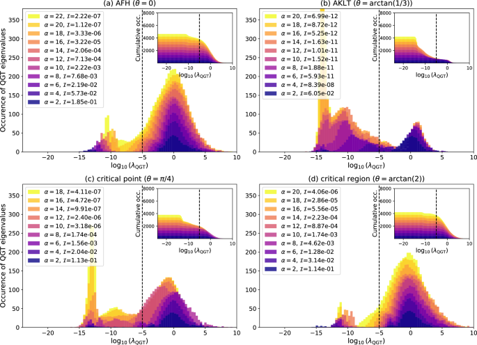
The spectra of the QGT are shown for the four phases (a–d) (corresponding to the four marked points in Fig. 1) after convergence of the infidelity minimization of the neural quantum state (NQS) w.r.t. the exact ground state of the spin-1 BLBQ chain with length L = 10, for various values of hidden layer density α. The infidelities (I) of the converged NQSs are shown in the legends. The QGT eigenvalues are shown in ({log }_{10}) scale. The insets show the cumulative distribution of the eigenvalues (number of eigenvalues exceeding the value on the x axis) for each case. The dashed line marks the cutoff 10⁻⁵, used for computing the rank d_r.

Full size image

In summary, we have performed a large number of numerical experiments to find ground states in various phases of the spin-1 BLBQ chain using a 1-layer NQS ansatz (Eq. (11)). We perform a supervised learning procedure, where we minimize the infidelity of the NQS w.r.t. the exact ground state (Eq. (2)). By increasing the hidden layer density α of the network, we achieve NQS approximations with greater accuracy, sometimes even reaching numerical precision (I ≤ 10⁻¹¹). The increase in the NQS accuracy is accompanied by an increasing QGT rank (and the related quantity d_r/d_q). In contrast, we sometimes observe a premature saturation in the NQS accuracy, where the NQS infidelity does not decrease further with an increase in α. In this regime, the QGT rank (or d_r/d_q) saturates around a given value or grows very slowly, for NQS optimizations with different α. This provides strong evidence that the local representation power of an NQS ansatz can be characterized using the QGT rank (or the ratio d_r/d_q) at convergence, within a given optimization scheme.

We interpret the above observations as follows. The rank of the QGT measures the number of directions in the Hilbert space that can be accessed by an infinitesimal change of the parameters. More precisely, the QGT rank (d_r) gives the dimension of the tangent space around the optimized NQS upto a constant (pm{1}), arising from the subtraction of the rank-1 term from the Gram matrix (w.r.t. the tangent space) in (Eq. (6)). Therefore a higher d_r suggests that the NQS ansatz had more freedom to reach a higher accuracy, given a particular optimization scheme. Whereas a saturation in d_r, with an increase in α, limits the ability of the NQS to leverage the additional parameters for improving its accuracy, and hence leads to a premature saturation of the NQS accuracy. We identify this as a practical limitation to reach universal representability for the given NQS optimization. In such a case, the QGT spectrum mostly shows an increase in zero eigenvalues, corresponding to the redundant directions around the optimized NQS ansatz in the parameter space. It is important to note that our results do not suggest a breakdown of the universal representation theorems and rather demonstrate situations where practical limitations in the NQS optimization limit the accuracy of the NQS approximation with increasing width of the NN.

Such observation of redundant directions is consistent with established findings in the ML literature, which show that a substantial number of directions in the parameter space are redundant^20,21. This is in contrast to tensor network ansätze, where each variational parameter contributes to the entanglement entropy of the variational ansatz²⁵, systematically improving the approximation for the ground state. Nevertheless, our analysis of the QGT rank/spectrum can help diagnose a practical limitation to reach universal representability. When this happens, in most cases a premature saturation of the converged infidelity is accompanied by a saturation of the QGT rank (or d_r/d_q), with an increasing width of the NQS ansatz. In a few cases for L = 12, we observe that d_r/d_q does not fully saturate when the infidelity does, but rather grows at a slower rate than the number of parameters in the NQS ansatz. In the former case, the optimized NQS only adds redundant directions in its neighborhood as its width increases. In the latter case, the optimized NQS ansatz is very less sensitive to an increasing dimension of the relevant manifold, suggesting that the newly added directions only marginally improve the NQS approximation.

A premature saturation of the converged infidelity with a growing network width can arise from two independent factors: (i) the limited expressivity of the specific NQS architecture to represent a given ground state, or (ii) the inability of the optimization method to reach the global minimum of the cost function, or from a combination of the two. Although our analysis using the QGT rank can quantify the practical efficiency of a converged NQS ansatz and can identify when a practical limitation to reach universal representability happens within a given optimization scheme, it cannot precisely determine whether the premature saturation occurs due to the factor (i) or (ii). A saturation of the QGT rank at d_r < d_q (as commonly observed in cases of premature saturation of the converged infidelity) can be caused either by using a badly configured ansatz with redundant parameters, or by an inefficient optimization scheme.

Nevertheless, a compelling application of our analysis lies in characterizing different methods of encoding the input for a given NQS architecture. This involves an inspection of the rank of the QGT at initialization for different encodings, and choosing the encoding with the highest rank of the QGT, which would ensure that the chosen ansatz is the easiest to optimize.

To summarize the performance of the NQS ansatz across the four phases of the spin-1 BLBQ chain, we note that the NQS represents the ground states in the AKLT phase and the critical point at θ = π/4 with a lower value of d_r/d_q than that in the AFH phase and the critical phase at (theta =arctan (2)), for a given accuracy. The NQS approximation for the AKLT state performs the best, exhibiting the lowest QGT rank d_r, suggesting that it is the simplest state to be represented by the given NQS ansatz. Furthermore, the AKLT state is also the state with the simplest non-trivial entanglement structure, since it can be represented exactly as an MPS with bond dimension χ = 2⁴⁷. The NQS approximation for the critical phase at (theta =arctan (2)) has the largest QGT rank d_r. Moreover, it is interesting to note that the NQS approximation for the ULS critical point at θ = π/4 has a lower d_r/d_q than the AFH state despite having a higher bipartite entanglement entropy⁴⁸. This may be due to the fact that the Hamiltonian at the ULS point has an enhanced SU(3) symmetry^39,50, which requires further investigation.

Furthermore, an interesting question is how the converged infidelity and the QGT rank vary with network width under different optimization schemes. To investigate this, we also conducted the infidelity minimization for the AFH and the AKLT phases with another algorithm: a combination of ADAM⁶³ and YOGI⁶⁴ optimization (see supplementary Note 7), which are adaptive gradient-based optimizers that usually perform well for stochastic gradient descent (SGD). We found that the NQS approximations with ADAM+YOGI optimization were generally less accurate at large network widths than those obtained using NGD (see supplementary Fig. 7d–f). In most cases, the ADAM+YOGI optimization led to minimal improvement of the NQS approximation with increasing network width, which appeared nearly frozen unlike in the case of NGD optimizations. However, the behavior of the QGT rank with α was similar across the two optimization schemes, with d_r eventually saturating with α (see supplementary Fig. 7a–c). In summary, the NGD optimizations proved to be significantly more effective in finding accurate NQS approximations.

In conclusion, we have introduced the notion of the dimension of the relevant manifold around a converged NQS, defined as the rank of the QGT d_r, and have proposed the ratio d_r/d_q as an indicator to characterize the local representation power of an NQS ansatz within a given optimization scheme. We have also demonstrated the emergence of a practical limitation to reach universal representability, using the above indicator, which suggests that practical calculations with NQS-based ansätze can differ considerably from the asymptotic behavior predicted by universal representation theorems. However, it is important to note that our analysis holds when the QGT can be estimated exactly. In practical VMC computations, the empirical estimate of the QGT, or the neural tangent kernel (NTK)¹⁷ for NQS ansätze with a large number of parameters, is usually biased when sampled using wavefunction amplitudes⁵¹. As a result, the rank of the empirically estimated QGT/NTK does not give a reliable measure of the dimension of the relevant manifold. We leave for future work to explore the relation between an empirically estimated QGT/NTK and the dimension of the relevant manifold around a converged solution.

We use a modified version of the RBM, adapted for spin-1 systems¹⁵, as the NQS ansatz ({psi }_{theta }(sigma )={sum}_{h}exp left[{{{mathcal{E}}}}(sigma ,h)right]), where

is the energy function of the spin-1 RBM. Here θ = {{a_i}, {A_i}, {b_i}, {w_ij}, {W_ij}} is the set of all 2L + M + 2ML complex parameters of the spin-1 RBM, L is the number of sites in the spin chain (number of units in the visible layer), M = αL is the number of units in the hidden layer, h_i = ±1 is the ith hidden unit, and σ = {σ_i} denotes a spin-configuration on the lattice. Note from Eq. (11) that the NQS ansatz given by the spin-1 RBM is holomorphic, i.e., ψ_θ(σ) depends only on θ, and not on θ^*, i.e., ∂ψ_θ/∂θ^* = 0. We remark that the above NQS ansatz intrinsically uses the (log (cosh (cdot ))) activation function, which has branch cuts in the complex plane, making universal representability proofs^9,12 directly inapplicable for complex parameters. While splitting complex parameters into real and imaginary parts resolves this, universal approximation for complex activation functions remains largely unexplored except in a few cases⁶⁵, though it is generally believed to hold in the large-parameter limit⁶⁶.

We use the above NQS ansatz (Eq. (11)) to represent the ground states of the spin-1 BLBQ chain in different phases. We use the infidelity measured w.r.t. the exact ground state as the loss function, for optimizing our NQS ansatz.

Infidelity optimization

For the infidelity minimization, we use the loss function given by the infidelity of the NQS w.r.t. the exact ground state (| Omega left.rightrangle),

where (theta in {{mathbb{C}}}^{N}). The loss function is minimized using the NGD algorithm^{31,32,58,59,60}. In the NGD method, the parameters of the ansatz are updated as

where G is the QGT, η is the learning rate, ϵ is a small regularization constant that prevents the inverse from diverging, and F_ν is the conjugate gradient of the loss function,

We compute the infidelity, the conjugate gradient, and the QGT exactly, by summing over the basis of the total S_z = 0 sector of the Hilbert space. For better performance, we adjust the regularization constant ϵ during the course of the optimization. We also tested the infidelity minimization with a combination of ADAM⁶³ and YOGI⁶⁴ optimizers (see supplementary Note 7), but we found that the convergence was unstable, and the solutions were significantly worse compared to those found with the current strategy. We defer an in-depth discussion on the optimization procedure to Supplementary Note 3.