Efficient equivariant model for machine learning interatomic potentials

In the field of computational materials, calculating interatomic potentials is critical for obtaining energy and related physical quantities such as forces and atomic trajectories. Computational methods that use pre-fitted empirical functions to form interatomic potentials, such as classical molecular dynamics (MD), provide very fast but less accurate material-property calculations. Meanwhile, methods based on high-fidelity quantum-mechanics calculations, such as density functional theory (DFT) and ab initio molecular dynamics (AIMD), offer highly accurate energies and forces but require high computational costs.

To address the above dilemma, deep learning techniques, such as graph neural networks (GNNs), have been proposed for predicting interatomic potentials^1,2,3,4 or DFT Hamiltonian^5,6,7,8 in speed while preserving quantum mechanics-level accuracy. These models can be mainly divided into two categories: invariant models^{9,10,11,12,13,14,15}, such as CGCNN¹⁶, SchNet¹⁷, MEGNet¹⁸, ALIGNN¹⁹, and M3GNet³, and equivariant models^{20,21,22,23,24}, such as MACE¹, NequIP², ScN²⁵, eScN²⁶, and DeepRelax²⁷. To represent the molecule or crystal structure, GNNs typically use a graph where nodes are atoms and edges are bonds between atoms. Atomic interactions are then simulated by applying graph convolution operations on the graph, where an atom can access its neighboring atoms during this process (Fig. 1a).

a A typical GNN workflow is illustrated, emphasizing how GNNs can include a wider range of interactions (or message passing) by stacking multiple layers to extend the accessible radius. b, c, and d underscore the importance of integrating structural features into GNNs, which include: b distance only, c both distance and angles, and d all distance, angles, and dihedral angles. e, f, and g elucidate the concepts of invariance and equivariance within the context of energy and force prediction.

Full size image

Currently, the most widely used GNNs are designed with architectures that are invariant to transformations from the Euclidean group E(3), ensuring consistent output for energy relative to translations, rotations, and reflections. This is achieved by leveraging invariant features, such as bond lengths and angles, which remain constant under these transformations. Early models like CGCNN¹⁶, SchNet¹⁷, and MEGNet¹⁸ primarily incorporate bond lengths, leading to challenges in distinguishing structures with identical bond lengths but different overall configurations (Fig. 1b). Later iterations, like DimeNet²⁸, ALIGNN¹⁹, and M3GNet³, improve upon this by integrating bond angles. Despite this improvement, they still struggled to differentiate between structures sharing the same angles (Fig. 1c). Recent models, such as GemNet²⁹ and SphereNet³⁰, propose considering dihedral angles in GNNs to unambiguously recognize the local structures (Fig. 1d). It is worth noting that distance and angular features are invariant representations which are only used to keep the geometric symmetry of crystals with respect to E(3) transformations rather than utilize the geometric symmetries in a more profound manner for increasing the prediction accuracy and the sample efficiency. Actually, the idea to leverage crystal symmetry for effectively describing the electron wave function and material properties was proposed a century ago. Felix Bloch demonstrated a translation-symmetry-based structural function to maintain the equivariance of wave functions in 1928. Such an equivariant idea in crystals with periodic structures in 3D space provides a powerful framework for accurately understanding the material properties and significantly reduces the cost of computation, opening a new era for computational material science. Figure 1e–g offer a concise elucidation of invariance and equivariance in the context of predicting energy and forces.

In this work, we integrate equivariance into GNNs for actively exploiting crystal symmetries and offering a richer geometrical representation compared to their invariant counterparts. Most importantly, our equivariant network is efficient, incorporating only scalar and vector features in a manner that preserves symmetry. Our efficient equivariant interaction graph neural network (E²GNN) is different from previously equivariant GNNs which are based on high-order functions, such as the spherical harmonic function. While these high-order functions have been associated with increased accuracy compared to invariant GNNs, they typically come at the cost of increased computational expense^{1,2,22,23,24,25,26,31,32,33,34,35}. For example, cutting-edge models like NequIP², MACE¹, ScN²⁵, and eScN²⁶ employ tensor product operations to combine input features and filters in an equivariant manner, which is computationally demanding in practice^25,26,36.

Our model aims to achieve both accurate and efficient predictions for interatomic potentials and forces. Specifically, we assign each node both scalars and vectors to represent equivariant features. E²GNN combines these entities in a symmetry-preserving fashion to maintain equivariance. Equivariant E²GNN surpasses scalar-only invariant models^16,17,18 in accuracy and generalization ability. It also offers an efficient structure compared to high-order tensor models^1,2,25. We also conduct MD simulations using E²GNN potential across solid, liquid, and gas systems. E²GNN can achieve the ab initio MD accuracy with high computational efficiency across all examined systems, showing its accuracy and efficiency.

Network architecture

The proposed E²GNN aims to enhance GNNs by incorporating equivariance, offering a richer geometric representation while retaining an efficient model. Each node in E²GNN is assigned scalars and vectors to represent invariant and equivariant features, respectively. This approach is similar to PaiNN³⁷ and NewtonNet³⁸, but with a more powerful message update scheme and global interaction modeling.

E²GNN gradually updates the node representations through four key processes: global message distributing, local message passing, local message updating, and global message aggregating, as illustrated in Fig. 2a and detailed in Fig. 2b–d. The local message-passing phase aggregates information from neighboring nodes to simulate two-body interactions. The local message updating phase integrates F scalars and F vectors within a node to update node representations. The global message aggregating and distributing phases promote long-range information exchange by maintaining a global scalar and vector.

a E²GNN uses message distributing, message passing, message updating, and message aggregating to iteratively update node representations. b E²GNN consists of T layers. c The message passing phase. d The message updating phase. The number of features after each operation is annotated in gray.

Full size image

Problem definition

In this work, the atomic structure is represented as a 3D interaction graph ({mathcal{G}}=({mathcal{V}},{mathcal{E}},{mathcal{R}})), where ({mathcal{V}}) and ({mathcal{E}}) are sets of nodes and edges. ({mathcal{R}}) are sets of 3D coordinates of nodes. Each node is connected to its closest neighbors within a cutoff distance D with a maximum number of neighbors N, where D and N are predefined numbers. Each node ({v}_{i}in {mathcal{V}}) has its scalar feature ({{bf{x}}}_{i}in {{mathbb{R}}}^{F}), vector feature ({overrightarrow{{bf{x}}}}_{i}in {{mathbb{R}}}^{Ftimes 3}) (i.e., retaining F scalars and F vectors for each node), and 3D coordinate ({overrightarrow{{bf{r}}}}_{i}in {{mathbb{R}}}^{3}). The scalar and vector features can be updated during training. We set the number of features F as a constant throughout the network. The scalar feature is initialized to an embedding only dependent on the atomic number as ({{bf{x}}}_{i}^{(0)}=E({z}_{i})in {{mathbb{R}}}^{F}), where z_i is the atomic number and E is an embedding layer that takes z_i as input and returns a F-dimensional feature. This embedding is similar to the one-hot vector but is trainable. The vector feature is set to ({overrightarrow{{bf{x}}}}_{i}^{(0)}=overrightarrow{{bf{0}}}in {{mathbb{R}}}^{Ftimes 3}) at the initial step. We also define ({overrightarrow{{bf{r}}}}_{ij}={overrightarrow{{bf{r}}}}_{j}-{overrightarrow{{bf{r}}}}_{i}) as a vector from node v_i to node v_j. Norm ∥ ⋅ ∥ and dot product ⋅ are calculated along the spatial dimension, while concatenation ⊕ and Hadamard product ∘ are calculated along the feature dimension. Given a set of 3D interaction graphs, our goal is to learn a model f to predict the potentials and forces as (f({mathcal{G}})=(e,overrightarrow{{bf{F}}})), where (ein {{mathbb{R}}}^{1}), (overrightarrow{{bf{F}}}in {{mathbb{R}}}^{Mtimes 3}) and M is the number of nodes in ({mathcal{G}}).

Local message passing

In the t-th layer, during local message passing, a particular node v_i gathers messages from its neighboring scalar ({{bf{x}}}_{j}^{(t)}) and vector ({overrightarrow{{bf{x}}}}_{j}^{(t)}), resulting in intermediate scalar and vector variables m_i and ({overrightarrow{{bf{m}}}}_{i}) as follows:

Here, ({{bf{W}}}_{h},{{bf{W}}}_{u},{{bf{W}}}_{v}in {{mathbb{R}}}^{Ftimes F}) are learnable matrices. The functions λ_h, λ_u, and λ_v are the linear combination of Gaussian radial basis functions¹⁷. For the Eq. (2), the first term (({{bf{W}}}_{u}{{bf{x}}}_{j}^{(t)})circ {lambda }_{u}(parallel {overrightarrow{{bf{r}}}}_{ji}parallel )circ {overrightarrow{{bf{x}}}}_{j}^{(t)}) propagates directional information ({overrightarrow{{bf{x}}}}_{j}^{(t)}) obtained in the previous step to neighboring atoms, with (({{bf{W}}}_{u}{{bf{x}}}_{j}^{(t)})circ {lambda }_{u}(parallel {overrightarrow{{bf{r}}}}_{ji}parallel )) acting as a gate signal to control how many signals in the previous step can be preserved. We interpret the second term as the force exerted by atom j on atom i, where (({{bf{W}}}_{v}{{bf{x}}}_{j}^{(t)})circ {lambda }_{v}(parallel {overrightarrow{{bf{r}}}}_{ji}parallel )) is force magnitude and (frac{{overrightarrow{{bf{r}}}}_{ji}}{parallel {overrightarrow{{bf{r}}}}_{ji}parallel }) is the force direction. This is conceptually different from PaiNN’s message function, which uses ({overrightarrow{{bf{r}}}}_{ij}) instead of ({overrightarrow{{bf{r}}}}_{ji}). Subsequently, ({sum }_{{v}_{j}in {mathcal{N}}({v}_{i})}({{bf{W}}}_{v}{{bf{x}}}_{j}^{(t)})circ {lambda }_{v}(parallel {overrightarrow{{bf{r}}}}_{ji}parallel )circ frac{{overrightarrow{{bf{r}}}}_{ji}}{parallel {overrightarrow{{bf{r}}}}_{ji}parallel }) represents the total force exerted on atom i and is a linear combination of forces exerted on it by all other atoms. Figure 3a shows an example of how the F forces are calculated.

a An example explains how to calculate the intermediate vector representation ({overrightarrow{{bf{m}}}}_{1}). For the sake of simplicity, we ignore the first term of Eqn. (2). The f-th vector in ({overrightarrow{{bf{m}}}}_{1}) (i.e., ({overrightarrow{{bf{m}}}}_{1}^{f})) can be interpreted as the force exerted by neighboring atom j on atom 1, where ({w}_{j1}^{f}) is force magnitude and (frac{{overrightarrow{{bf{r}}}}_{j1}}{parallel {overrightarrow{{bf{r}}}}_{j1}parallel }) is the force direction. Subsequently, the total force exerted on atom 1 is a linear combination of forces exerted on it by all other neighboring atoms j. Note that the forces are calculated F times in parallel. b The update to ({overrightarrow{{bf{x}}}}_{1}^{f}) is achieved through a linear combination of F vectors within ({overrightarrow{{bf{m}}}}_{1}). This computation is performed in parallel F times to obtain ({overrightarrow{{bf{x}}}}_{1}).

Full size image

Local message updating

The local message updating phase aims to aggregate F scalars and vectors within m_i and ({overrightarrow{{bf{m}}}}_{i}), respectively, to obtain new scalar ({{bf{x}}}_{i}^{(t+1)}) and new vector ({overrightarrow{{bf{x}}}}_{i}^{(t+1)}), as shown in Fig. 3b. Specifically, the scalar representation ({{bf{x}}}_{i}^{(t+1)}) and vector representation ({overrightarrow{{bf{x}}}}_{i}^{(t+1)}) are updated according to the following equations:

where ⊕ denotes concatenation, ({{bf{W}}}_{s},{{bf{W}}}_{g},{{bf{W}}}_{h}in {{mathbb{R}}}^{Ftimes 2F}), and ({bf{U}},{bf{V}}in {{mathbb{R}}}^{Ftimes F}). The term (tanh ({{bf{W}}}_{g}({{bf{m}}}_{i}oplus parallel {bf{V}}{overrightarrow{{bf{m}}}}_{i}parallel ))) acts as a gate controlling how much invariant signal from the previous layer is preserved. This design allows for selective updating of node representations, which can help in preserving important features from the previous layers while incorporating new information.

Global message distributing and aggregating

In many GNN architectures, information primarily flows locally between directly connected nodes. While increasing the depth of GNNs can broaden receptive fields, it can also lead to optimization instabilities, such as vanishing gradients and representation oversmoothing. To facilitate a more effective global communication channel across the entire graph, we propose a global message distributing and aggregating scheme by creating a global scalar ({{bf{x}}}_{{mathcal{G}}}) and a global vector ({overrightarrow{{bf{x}}}}_{{mathcal{G}}}). Specifically, we initialize the global scalar and vector as ({{bf{x}}}_{{mathcal{G}}}^{(0)}in {{mathbb{R}}}^{F}) and ({overrightarrow{{bf{x}}}}_{{mathcal{G}}}^{(0)}=overrightarrow{{bf{0}}}in {{mathbb{R}}}^{Ftimes 3}), where ({{bf{x}}}_{{mathcal{G}}}^{(0)}) is trainable. The global message distributing operates before the local message passing, distributing the global scalar and vector at the current step to each node using the following equations:

where (phi :{{mathbb{R}}}^{2F}to {{mathbb{R}}}^{F}) refers to a multi-layer perceptron layer (MLP), and ({bf{W}}in {{mathbb{R}}}^{Ftimes F}) is a trainable matrix. After local message updating, the global scalar and vector are updated using the node representations at the current step with the following equations:

E²GNN is strictly equivariant to rotation and translation, as proven in SM Section 1. Its design also guarantees the extensivity of energy, i.e., the predicted energy of E²GNN is linear with respect to the simulation box size, as proven in SM Section 2.

Predicting potentials and forces

To predict the potential e, we utilize an MLP layer (phi :{{mathbb{R}}}^{F}to {{mathbb{R}}}^{1}). This layer learns atom-wise potentials ({e}_{i}in {{mathbb{R}}}^{1}) from the scalar representation ({{bf{x}}}_{i}^{(T)}), which is obtained at the last graph convolution layer (referred to as the T-th layer). The total potential is then calculated as the sum of the atom-wise potentials:

The forces are predicted using the vector representation ({overrightarrow{{bf{x}}}}_{i}^{(T)}) as (overrightarrow{{bf{F}}}={{bf{W}}}_{f}{overrightarrow{{bf{x}}}}_{i}^{(T)}), where ({{bf{W}}}_{f}in {{mathbb{R}}}^{1times F}). This approach offers the advantage of creating a efficient model by directly computing forces, which bypasses the computationally expensive tasks of calculating the gradient of the potential energy (first derivative) and the second derivative during backpropagation for model parameter updates. Although the directly predicted forces are not energy conserving, they can still facilitate MD simulations, especially when a thermostat is employed to regulate the temperature^36,39.

Implementation details

The E²GNN model is implemented using PyTorch. Experiments are conducted on an NVIDIA GeForce RTX A4000 with 16 GB of memory. The training objective aims to minimize the loss function defined as:

where ({e}_{n}^{l}) represents the ground truth energy of n-th sample, ({overrightarrow{{bf{F}}}}_{nmk}^{l}) is the ground truth force of k-th dimension of m-th atom in n-th sample. The variables N and M denote the sample size and the number of atoms in each sample, and α and β denote the weights assigned to the energy and force losses, respectively.

Model performance

We first evaluate E²GNN in the structure to energy and forces (S2EF) task using Open Catalyst 2020 (OC20) dataset⁴⁰. The purpose of this task is to predict energies and forces corresponding to each trajectory during structural relaxation. The OC20 dataset encompasses 1,281,040 density functional theory (DFT) relaxations with 264,890,000 single-point calculations and spans a vast range of materials, surfaces, and adsorbates. It has been reported that training a GNN model on the whole OC20 dataset requires hundreds or even thousands of days²⁶. Therefore, we only use a subset of it: OC20-200 K (N = 200, 000). The dataset is split into a training set and an internal validation set with a ratio of 8:2, where the internal validation set is used to select the best model for testing. Finally, the select models are tested on four external validation sets provided by the OC20 project: in Domain (ID), out-of-domain adsorbate (OOD Ads.), out-of-domain catalyst (OOD Cat.), and OOD Both (both the adsorbate and catalyst are not seen in the training set). Each external validation set contains approximately 1M data points. We compare E²GNN with seven representative baseline models: CGCNN¹⁶, SchNet¹⁷, MACE¹, PaiNN³⁷, PaiNN_Direct⁴¹, DimeNet++⁴², and GemNet-dT²⁹. PaiNN_Direct is a modified version of PaiNN designed for making direct force predictions. The hyperparameter configuration for each model is provided in SM Section 3. All models share the same training, internal validation, and external validation sets, and are trained to predict adsorption energy and per-atom forces simultaneously. The performance of the models is evaluated based on the mean absolute error (MAE).

From Table 1, we have two key observations. First, E²GNN achieves performance close to GemNet-dT and outperforms other baseline models. Second, PaiNN_Direct surpasses PaiNN, which aligns with previously reported results⁴³. Additional experimental results on a smaller subset, OC20-50 K, are available in SM Section 4.

Next, we compare the computational costs among E²GNN and five accurate models: MACE, PaiNN, PaiNN_Direct, DimeNet++, and GemNet-dT. Figure 4 illustrates the model complexity in terms of training time, inference time, the number of parameters, and floating-point operations (FLOPs). It is worth noting that the number of parameters and FLOPs are estimated using PyTorch-OpCounter, which fails when applied to MACE. We have three key observations. First, E²GNN offers approximately ten times faster training and inference speeds than GemNet-dT and MACE, and about five times faster than DimeNet++ and PaiNN. Second, E²GNN has a similar computational cost to PaiNN_Direct but demonstrates better performance. Third, the computational cost of PaiNN_Direct is significantly lower than that of PaiNN. Considering that the main difference between PaiNN_Direct and PaiNN is how they compute forces, we can conclude that computing forces by taking the derivative of the energy with respect to positions is more computationally demanding.

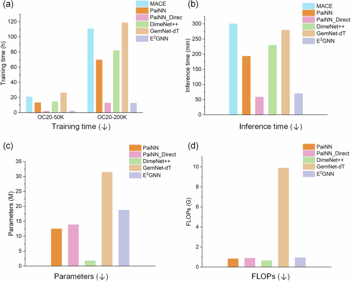
a Training time. b Mean inference time. c Number of parameters. d FLOPs.

Full size image

Figure 5 shows a Pareto front plot, with the two axes representing inference time and force MAE. The Pareto front highlights that our model achieves one of the best trade-offs between speed and accuracy among the benchmarked ML models. Overall, our results show that direct force prediction improves both efficiency and performance, consistent with previous studies^15,32,43. Besides the OC20 database, we compare E²GNN with other models on MD17 and ISO17 databases. Our E²GNN model also surpasses those benchmark models on these two databases (see SM Sections 7 and 8), showing the universality of E²GNN.

The x-axis represents inference time (min), while the y-axis shows force MAE (meV/Å). Models on the Pareto front, including our proposed model, demonstrate an optimal balance between computational efficiency and prediction accuracy.

Full size image

Ablation study

The novelty of E²GNN lies in two aspects: a novel message updating (NMU) scheme and the global message aggregating and distributing phases to promote long-range information exchange among atoms. To demonstrate the effectiveness of these strategies, we compare E²GNN with two baseline models: Vanilla and Vanilla + NMU. The Vanilla model excludes both the NMU scheme and the global message phases, using PaiNN’s message updating instead. The Vanilla + NMU model includes only the NMU scheme. As shown in Table 2, E²GNN notably outperforms both baseline models. Besides, it is worth noting that such two strategies are carried out on nodes rather than edges. This design choice offers a computational advantage because the number of nodes is typically significantly smaller than the number of edges in a graph. Note that the Vanilla model differs from PaiNN_Direct in several ways. Additional details are provided in SM Section 3.

Molecular dynamics simulations

Molecular dynamics simulations provide vital atomistic insights, but the accuracy versus efficiency trade-off has long been a challenge. Classical MD, which relies on empirical interatomic potentials, is computationally efficient but sacrifices accuracy. In contrast, AIMD, which integrates first-principles methods such as density functional theory, provides higher accuracy but at a high computational cost. Recently, machine learning-based force fields have emerged as a promising solution to enhance the speed of MD simulations by several orders of magnitude while maintaining quantum chemical accuracy.

To validate the interatomic potentials of our E²GNN model, we demonstrate that E²GNN performs competitively against established baseline models such as DeepPot-SE⁴⁴, SchNet¹⁷, DimeNet²⁸, ForceNet¹⁵, GemNet-T²⁹, GemNet-dT²⁹, and NequIP². We evaluate the models’ performance using the mean absolute error (MAE) of the radial distribution function (RDF), stability, and diffusivity. Our definitions of stability and diffusivity align with those used in MDSim³⁶. A simulation is considered “unstable” if deviations exceed predefined thresholds, leading to the sampling of highly nonphysical structures. Diffusivity measures the time-correlation of translational displacement. For detailed experimental settings and metrics, refer to SM Sections 5 and 6.

We consider three systems: LiPS (solid), H₂O (liquid), and CH₄ (gas), as depicted in Fig. 6a, where the data for H₂O and CH₄ (gas) are collected in-house to assess E²GNN’s effectiveness in liquid and gaseous systems. We conduct a 50-picosecond simulation for each system, starting from a randomly selected test configuration. The training, validation, and testing sets for the LiPS system are consistent with those used in MDSim. The results for the LiPS system are summarized in Table 3. Although the forces predicted by E²GNN are not from the widely used energy-conserving method, the MD simulation performance remains competitive with that of energy-conserving models. Figure 6b, c shows the h(r) and RDF for AIMD and E²GNN across the three systems, revealing their strong alignment. Using the same stability criterion as for the LiPS system, E²GNN also demonstrates consistent stability throughout the 50 ps simulations in the H₂O (liquid) and CH₄ (gas) systems. These results highlight E²GNN’s potential as a crucial tool in computational materials science.

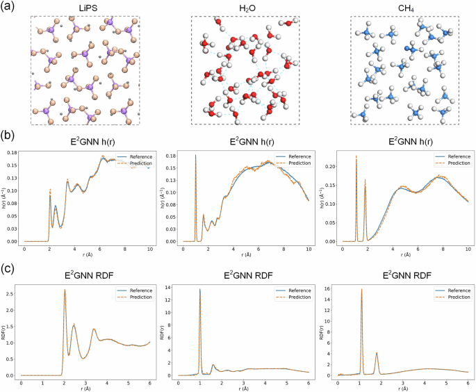
a An overview of the three benchmark systems. b h(r) for trajectories predicted by the E²GNN. c RDF for trajectories predicted by E²GNN.

Full size image

Since the introduction of global entities can potentially lead to inaccuracies in scenarios where distant parts of the system are improperly influenced, we further tested E²GNN on a larger system consisting of 2241 atoms. The results presented in SM Fig. S2 show that the RDF remains consistent between the supercell ML trajectory and the DFT trajectory. This suggests that long-range communication between atoms, introduced by the global node, does not significantly affect the system’s physical behavior in terms of pairwise distances. Further discussions are available in SM Section 9.

We develop an accurate and efficient equivariant graph neural network for predicting interatomic potentials and forces. The efficient nature of E²GNN comes from two factors: direct force predictions and modeling only two-body interactions. E²GNN consistently outperforms the prediction performance of the representative baselines across diverse molecular and crystal datasets. Moreover, E²GNN achieves the precision of ab initio MD while maintaining high computational efficiency in simulations involving gas, liquid, and solid systems. Despite its advancements, we would like to say two limitations. First, the introduction of global entities may lead to inaccuracies in certain scenarios where distant parts of the system are incorrectly influenced by global changes, such as two “isolated” molecules in a big box without interaction between them. Second, the forces are predicted directly, which is not energy-conserving, and a thermostat is needed to regulate the temperature^15,36.