EFTGAN: Elemental features and transferring corrected data augmentation for the study of high-entropy alloys

In recent years, artificial intelligence (AI) has become an important driver of advanced material research and development¹. Machine learning, as an important AI tool, has been widely used in materials design². By accomplishing regression, classification and clustering tasks for material science, machine learning methods provide viable solutions for predicting material properties and screening potential candidate materials³. Over the past few decades, machine learning has accomplished accurate predictions of the properties of a wide range of important materials, including mechanical properties of alloys^4,5, bandgap energies⁶, photovoltaic materials⁷, superconducting critical temperatures⁸, etc. Generally, constructing a machine learning model requires selecting descriptors as inputs that conform to the underlying physical properties. These descriptors are typically stoichiometric attributes, composition, lattices, elemental properties such as electronegativity, etc^9,10,11,12. With ensemble learning algorithms such as XGBoost¹³, Random Forest¹⁴, or deep learning algorithms with embedding¹⁵, these descriptors are able to achieve a high level of accuracy on specific problems. The inputs are all quantities that can be simply obtained. This facilitates the model to make a large range of predictions, and also helps to find the intrinsic connection between descriptors and outputs¹⁶. However, for materials with complex structures, large lattice distortions or properties with strong structural correlations, descriptors based on simple material properties can not fit well. An effective approach to this problem is to use accurate structures as model inputs. The use of molecular structure as a descriptor is a viable method for screening high-performance organic materials^17,18,19. For materials with periodic lattices, deep learning networks based on graph models has recently been applied to them^20,21,22. The graph model is able to convert the exact crystal structure into a graph represented by atomic properties and bond properties, and the deep learning network uses the large amount of information in the graph to accurately fit the material properties in various systems. The graph neural models exhibit much higher performance than ensemble learning.

Large-scale screening of alloys using traditional calculation methods is particularly difficult due to the diversity of alloy elemental compositions. The application of machine learning in the study of alloys has proven particularly important in driving advances in a variety of materials, including metallic glasses, high-entropy alloys (HEAs), magnets, superalloys, shape-memory alloys, catalysts, and structural materials²³. Among them, HEAs have attracted attention due to not only their excellent mechanical properties, but also their unique magnetic and electrical properties^24,25,26. The use of machine learning methods can avoid the computational difficulties associated with large supercells in density functional theory (DFT). A number of machine learning models have been applied to HEAs, especially for phase classification²⁷ and prediction of mechanical properties²⁸. In addition, new progress has been made in the prediction of energies, magnetic moments and other microscopic properties of HEAs^29,30. In the practical application, machine learning has completed the screening of HEAs for catalyst of water splitting³¹. These properties, which are strongly correlated with structures, often require the use of graph neural networks. Data-driven machine learning methods, however, often require a sufficiently large number of training samples. The complexity of DFT calculations for HEAs also limits the size of the accurate structured data that can be used for graph neural networks. The need for accurate structures as input also limits the model to large-scale predictions.

Generative Adversarial Networks (GAN) are a powerful machine learning tool for generating new data samples³². Using the GAN model to generate new data as data augmentation for machine learning can solve the problem of insufficient data for HEAs³³. The classical GAN model architecture consists of two neural networks – a generator and a discriminator. The generator is trained to generate data, while the task of discriminator is to determine whether these samples are real or generated. Information Maximizing Generative Adversarial Networks (InfoGAN) that also has a classifier is a variant of GAN³⁴. This classifier is used to extract additional information from the data to enable the generation of state-specific data. The generation of structures under specific composition by the InfoGAN model can be helpful for the practical use of graph neural networks. In order to ensure the data generated by the InfoGAN model accurate and effective, we developed a framework based InfoGAN algorithm: Elemental Features enhanced and Transferring corrected data augmentation in Generative Adversarial Networks(EFTGAN). In the EFTGAN model, we use elemental convolution graph neural networks (ECNet) to extract elemental features suitable for describing the predicted targets from the atomic and structural information of the crystal³⁰. These features will be transferred to the InfoGAN model, which is used to generate new elemental features with predicted targets instead of generating the original crystal structure. With elemental convolution, the elemental features not only extract the knowledge of the crystal structure and atomic information, but also can be updated by learning the intrinsic properties of predicted target, making them highly relevant to the predicted targets. This correlation improves the credibility of the new data generated by the InfoGAN model based on similarity. These generated new data will be used for data augmentation to improve the prediction accuracy of neural networks with small data set. We propose an iterative approach to ensure that data augmentation is effective.

In this paper, we propose the EFTGAN machine learning model and apply it to high-entropy FeNiCoCrMn (Cantor alloy) and FeNiCoCrPd alloy systems. We predict the formation energy, magnetic moments, and root mean-square displacement (RMSD) of HEAs. In order to prevent too much generated data from decreasing the prediction accuracy of the real data, we use transfer learning to input the generated data into the prediction model. EFTGAN outperforms the ECNet model without data augmentation in various properties. Meanwhile, the elemental features of unknown-structure materials generated using the EFTGAN model can be directly input into the prediction model, which greatly enhances the prediction ability of the ECNet model. This allows us to achieve a wide range of predictions without structure data for HEAs and maintain accuracy consistent with graph neural networks in which the structure data are available. These results help us to better understand the properties of HEAs and enrich the physics of HEAs.

The EFTGAN model

The workflow of our model starts with a complete ECNet model, as shown in the green block of Fig. 1. The ECNet model can be divided into two parts, elemental convolution and multilayer perceptron. Elemental convolution allows extraction of information about each atom from an undirected graph representing the crystal structure, and transforms atom information into global elemental features based on atomic species. The multi-layer perceptron is responsible for predicting target and updating the elemental features through backpropagation. We extract elemental features from the trained ECNet model and combine them with the original target values as shown in the purple block of Fig. 1. The elemental feature vector is represented as a color band, where red and blue denote positive and negative values. In the blue Block, the generator of InfoGAN model is used to generate new data similar to the element features and targets. The input to the generator contains elemental composition, rather than just noise. The classifier and discriminator of InfoGAN model are then used to determine whether the new data generated by the generator has the correct elemental composition and whether it is real or fake. The network structure of generators, discriminators and classifiers can be varied with the research target.

The green block is a ECNet model. The elemental convolution operation is used to extract the features of each element in the materials. The principal component analysis is used to downscale features to improve generator performance. The purple block is elemental features after downscaling. The blue block is InfoGAN model. The iteration use the multi-layer perceptron to predict the features generated by INfoGAN, returning the results to InfoGAN training.

Full size image

We use principal component analysis (PCA) to downscale the features before the elemental features are used to train the InfoGAN model. This is due to the fact that an excessively large data dimension can significantly degrade the performance of the generator relative to a small training set. This will result in the discriminator being able to distinguish between the generated data and the original data, but the generator and discriminator will not being able to be adversarial. It is worth mentioning that GAN generates new data based on the similarity of the new data to the original data. However, the relationship between features and properties is not completely similar, and the same properties may correspond to completely different features, which leads to poor extrapolation of GAN for target generation. In the EFTGAN model, we use elemental feature extraction and iteration to solve this problem. Elemental feature extraction can get elemental features that have some similarity with the properties. After the InfoGAN model is trained, we take only the generated features and predict targets with the generated features using a multi-layer perceptron trained with the original data. These data are added to the training set to update the InfoGAN model. This operation is repeated several times until the generated targets no longer change significantly. We also utilize similarity to improve the performance of generation. Generating several correlated targets together can improve target generation accuracy. For this reason, the ECNet model used to extract elemental features should also be multitasking, which improves the performance of the prediction. When using generated data for data augmentation, we use transfer learning to prevent too much generated data from deteriorating the prediction accuracy of the original data. We first train the multi-layer perceptron using the generated data, fixing the first two layers of the network unchanged, and then updating the remaining network with the original data.

Application in HEAs

For the application of the EFTGAN model in HEAs, we focus on FeNiCoCrMn/ Pd quinary HEAs and their binary, ternary, and quaternary subsystems. These HEA systems have exceptional strength and ductility at high temperatures^35,36. In the data set of this work, FCC and BCC single-phase solid solutions (SPSS) have the same number. And each data set contains 211 data, of which 42 are binaries, 64 are ternaries, 49 are quaternaries and 56 are quinaries³⁷. In order to study the properties of these alloys, we use the EFTGAN model to predict the total energies (E_tot), the mixing energies (E_mix), the formation energies (E_form), magnetic moments per atom (m_s) and magnetic moments per cell (m_b) and root-mean-square displacement (RMSD). The mixing energy of an HEA structure in m SPSS (m = FCC or BCC) is calculated as: ({{rm{E}}}_{{rm{mix}}}={{rm{E}}}_{{rm{tot}}}^{{rm{m}}}-{sum }_{{rm{i}}}{{rm{c}}}_{{rm{i}}}{{rm{E}}}_{{rm{i}}}^{{rm{m}}}), where ({{rm{E}}}_{{rm{tot}}}^{{rm{m}}}) is the total energy of the HEA, ({{rm{E}}}_{{rm{i}}}^{{rm{m}}}) is the total energy of the simple substance at 0K in m SPSS, and c_i is the ratios of each constituent element in the special quasirandom structure (SQS) structure used to model the HEA. The formation energy of an HEA structure is calculated as: ({{rm{E}}}_{{rm{form}}}={{rm{E}}}_{{rm{tot}}}^{{rm{m}}}-{sum }_{{rm{i}}}{{rm{c}}}_{{rm{i}}}{{rm{E}}}_{{rm{i}}}^{0}), where ({{rm{E}}}_{{rm{i}}}^{0}) is the total energy of the simple substance in its ground state. In the process of improving the performance of the model through multitasking, we find that multitasking to learn the three attributes E_tot, E_form and E_mix improves the quality of extracted features³⁰. m_b can be considered as m_s multiplied by the number of atoms in the cell, and there is a high linear correlation between the both. So performing multi-task learning not only is beneficial to improve the quality of features, but also improves the accuracy of the GAN generated target. Since there is no significant correlation with either energy or magnetic moments, RMSD alone is trained as a single-task model. In addition, in order for the model to better distinguish the differences between the FCC and BCC phases, we train the GAN networks separately for both phases.

For the performance analysis of the EFTGAN model, we show feature correlation analysis and iterative effect in Fig. 2. We have calculated the Pearson coefficient between the mean, variance, standard deviation of the elemental features((bar{{rm{F}}}), D(F), σ(F)), atomic radii weighted according to elemental ratios(R_x), weighted electronegativity(e_x), cell volume(V_c), (bar{{rm{A}}}) and σ(A) to represent the correlation³⁸. The format of elemental features(F) is shown in Fig. S1 of the Supplementary Material. A is the sum of reciprocals of distances of an atom from other atoms divided by the atom number in one cell. (bar{{rm{A}}}) and σ(A) represent the mean and standard deviation of A over atoms of the same element in one cell. As shown in Fig. 2a, the Pearson coefficient ranges from −1 to 1, where 1 represents absolute positive correlation and -1 represents absolute negative correlation. There is a strong correlation between the elemental features and R_x, e_x, V_c, (bar{{rm{A}}}) and σ(A) which proves that the feature extraction is able to obtain the elemental and structural information well. Specifically, the correlation between σ(F) and σ(A) demonstrates that elemental features can represent the variations in the local structure for atoms of the same element. The effect of the iteration time on the coefficient of determination (R²) between the predicted targets generated by the GAN and the DFT values is shown in Fig. 2b. As the iteration time increased, the R² for each target grows from 0.6 to more than 0.82. After the five iteration, GAN can be used as a data generator for data augmentation.

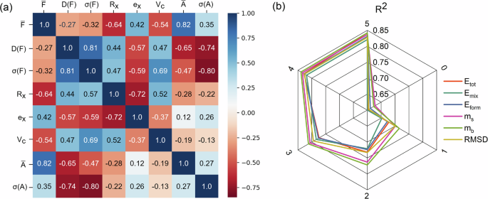
a shows the correlation of elemental features with elemental and structural information. Blue areas indicate negative correlation and red areas indicate positive correlation. b shows the effect of iteration on the prediction performance of GAN. The numbers 0–5 represent the times of iteration.

Full size image

We show in Table 1 the predictive performance of different models for each target using R² of the model test set. We also list the results for the ECNet model without EFTGAN data augmentation. Whether it is for properties such as E_tot, E_form, which are closer to global properties, or RMSD, which is more relevant to local atomic positions, the EFTGAN model outperforms the original ECNet model in all six predicted targets. This shows the universality of our data augmentation method, and the transfer of elemental features is a powerful way to accomplish data augmentation for completely different properties. In addition, we list the performance of the model for predicting E_form in ref. ³⁹. This model proposes a descriptor based on Voronoi Analysis and Shannon Entropy (VASE). In contrast, our EFTGAN model still has higher accuracy, suggesting that our input descriptors obtained by elemental feature extraction have better performance compared to descriptors found manually through logic.

Another important ability of the EFTGAN model is to achieve large-scale screening without structures. In the ECNet model, the input to the model is a graph containing information about the positions of the crystal atoms, which means accurate atom positions are required for property prediction. In contrast to the ECNet model, we are able to generate elemental features in any elemental composition for prediction of multi-layer perceptron in the EFTGAN model. We generate elemental features for the elemental composition of the data in the test set and predict the properties corresponding to these features, obtaining the prediction accuracy of the EFTGAN model without structural information inputs, as shown in the EFTGAN FCC and EFTGAN BCC columns of Table 1. ECNet FCC and ECNet BCC columns, on the other hand, show the performance of multi-layer perceptrons trained with weighted elemental vectors extracted from the ECNet model as descriptors. The EFTGAN model has better performance in all conditions and the performance difference with the case with structured inputs is very small. The ECNet FCC and ECNet BCC models, on the other hand, have a large performance gap with the original ECNet model, especially in the prediction of RMSD, which is closely related to atomic local information. This shows that simple weighted averaging of elemental vectors does not respond well to the local differences brought about by different element compositions, while the elemental features generated by the EFTGAN model are able to respond to this difference to some extent. The training time for the ECNet model and the EFTGAN model is essentially the same. For a HEA structure that contains more than 100 atoms, the EFTGAN model requires only one millionth of the time of the ECNet model to achieve the same accuracy for prediction. In addition, the prediction accuracy of the FCC phases is higher than that of the BCC phases in all models, due to the fact that the BCC phases generally have larger lattice distortions and larger RMSDs in our data, and thus the effects of local properties are more significant. Our EFTGAN model is also able to reduce this disparity. In addition, increasing the dimension of elemental features after PCA downscaling can also reduce this problem. When we increase the dimension from 32 to 40, the R² of E_form for BCC increases from 0.937 to 0.941. 32 is the dimension in which the entire model reaches its highest accuracy.

The parity plots in Fig. 3 show the comparison of the DFT calculations with the EFTGAN model predictions for the six properties of the FeNiCoCrMn/Pd alloys on the training, validation, and test sets. We observe that the EFTGAN model has good prediction performance. In this work, the hyperparameters of the model are determined when the prediction performance of the validation set is optimal. This may lead to poor prediction performance outside the range of validation set. The difference in data distributions among training, validation, and test sets are also shown in Fig. 3. One can observe that the prediction performance remains comparable, even when the data distributions of the validation and test set are not similar. This shows that the high performance of the EFTGAN model does not come from overfitting to the validation set.

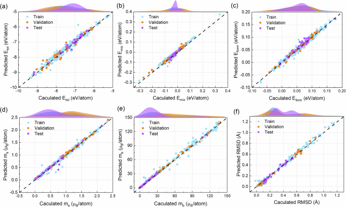
a E_tot; b E_mix; c E_form; d m_s; e m_b; f RMSD. The blue, orange, and purple points are samples from training, validation, and test data sets, and their data distributions are shown at the top of the parity plots.

Full size image

To intuitively show the generalization ability of the EFTGAN model, we calculate verifying alloy data located far from the internal range of the original data set. We calculate structures, E_form and m_s for the MnFeCo ternary FCC system. The elemental composition of these alloys are shown in Fig. 4. The blue points are compositions in the original data set and the blue shaded area is the internal composition range of the original data set. The orange data for verifying the generalization ability are taken to be distributed uniformly. Approximately 20% of the orange points are situated outside the shaded area. We use the EFTGAN model to generate elemental features from composition and predict the E_form and m_s. Meanwhile, we use the ECNet model to predict properties using structure as input. We compare the differences between the two model predictions and the DFT calculations.

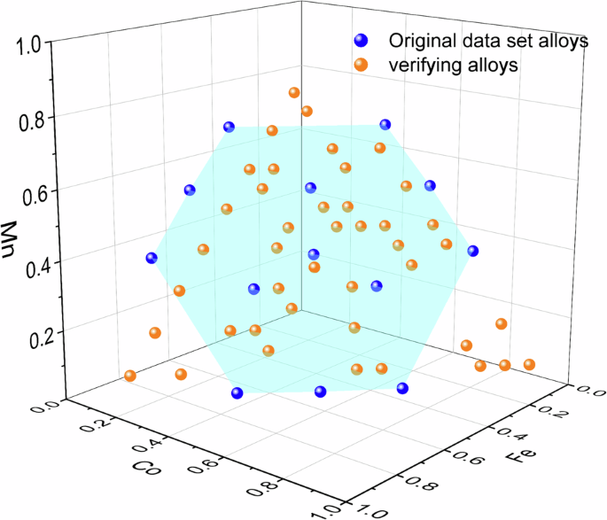
Blue points are compositions of binary ternary alloys for the MnFeCo system in the original data set, and orange points are compositions of verifying alloys in order to show the generalization ability. The shaded area is the internal range of the original data set.

Full size image

The comparison of prediction performance of the EFTGAN model and the ECNet model is shown in Fig. 5. Regardless of which model is used, the predicted values are in the vicinity of the DFT calculated values and reliable results are obtained using both methods. The predictions using the EFTGAN model to generate elemental features have performance comparable to the ECNet model, which is consistent with the results in Table 1. However, the prediction of the EFTGAN model does not need the structure information, which provides support for accurate large-scale prediction using EFTGAN model. More importantly, the results of generating feature predictions using the EFTGAN model are in the vicinity of the results of DFT calculations, regardless of whether the new alloy composition are far from the range of the training set. This shows that our EFTGAN model is able to generate effective elemental features outside the known range of the original data set. The variations between compositions are effectively captured without generating identical elemental features for different compositions. In general, using the EFTGAN model to generate elemental features is a useful way to reduce the computation involved in model prediction without losing much performance.

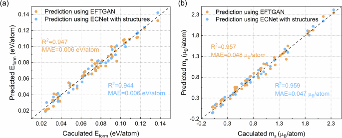
a E_form; b m_s. The blue points are the results predicted by the ECNet model with DFT calculated structures as inputs; the orange points are the results of the EFTGAN model by generating elemental features according to the elemental composition and then inputting them into the multi-layer perceptron. The blue and orange text shows the R² and mean absolute error (MAE) for the two methods, respectively.

Full size image

In the EFTGAN model, the most important hyperparameters are the elemental feature dimensions extracted by the ECNet model and the feature dimensions generated by the GAN model. Finding a balance between high accuracy and overfitting by adjusting the dimensionality of the elemental features is the focus of training the EFTGAN model. The effects of dimensions generated by the GAN model and dimensions extracted by the ECNet model on the prediction performance of the six properties are shown in Fig. 6. To prevent data leakage, the results of Fig. 6 are on the validation set. PCA finds the component with the highest variance in the high-dimensional space as the principal component. We use the cumulative variance percent to evaluate the difference between the downscaled features and the original features. The cumulative variance percent is 1 before downscaling. Figure 6a, b show the R² without data augmentation and cumulative variance percents after PCA downscaling, respectively. There is no significant decrease in the performance of models and all the cumulative variance percents are above 0.9 with 32 dimensions. This shows that PCA retains important components of the original features and the generated data is able to inherit important difference between elements from the original data. The prediction of the EFTGAN model reaches the best accuracy when the generated dimension of the GAN model is 32, at which point the adversarial between the generator and the discriminator reaches equilibrium. The extracted dimension of the ECNet model in Fig. 6a–d is fixed at 128. Figure S2 in the Supplementary Material shows the the variations under other extracted dimensions of the ECNet model, which follow a close trend. When the dimension generated by the GAN model is greater than 32, the performance of the discriminator is significantly greater than that of the generator, resulting in extreme proximity of the generated data to the original data and a significant decrease in prediction performance. This limitation is mainly determined by the amount of training data⁴⁰. On the contrary, when the dimension is less than 32, it does not degrade the generative ability of the GAN model. However, the fitting performance to the predicted target is degraded due to small input dimension and less information. Thus the generated dimension of the GAN model is fixed to 32. The effect of extracted dimensions by the ECNet model on the prediction performance when the generated dimension is fixed is shown in Fig. 6e, f. The predictions achieve best performance with extracted 128-dimensional features. The 128-dimension features contain more information compared to the extracted 32 or 64 dimensional features. In the PCA downscaling process, effective information is retained while noise is removed, leading to maximum prediction accuracy. In particular, we observe that the predictive performance of RMSD is optimal when the ECNet model extracts 256 dimension. This is due to the fact that RMSD is strongly correlated with local atomic properties, requiring higher dimension responses to more local information. While other models experience overfitting due to high dimensions. Therefore, we finally choose 32 and 128 as the dimensions for the GAN model generation and ECNet model extraction.

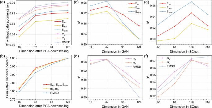
a shows the R² of models without data augmentation after PCA downscaling. b shows the cumulative variance percents of elemental features after PCA downscaling. c, d show the impact of the target feature dimensions generated by the GAN model after PCA downscaling on the prediction performance; e, f show the impact of the elemental feature dimensions extracted by the ECNet model on the results.

Full size image

In the EFTGAN model, the unique augmentation mode also provides performance improvements. In traditional data augmentation models, the generated data is trained together with the original data. Therefore, the size of the generated data set is limited in order to prevent the model from focusing on the generated data and ignoring the original data. In the EFTGAN model, we first train the model using the generated data and then use the trained network parameters as initial parameters and fix the parameters of the network front to train the original data. This augmentation mode is similar to transfer learning and we call it transfer augmentation. We show the effects of augmentation modes and size of augmentation samples to the R² of E_form in Table 2. As the size of augmentation samples increases, the performance of data augmentation quickly reaches a limit and begin to decrease. However, the performance of transfer augmentation rises to the limit and then remains stable. The transfer augmentation can use more augmentation samples to achieve much higher performance than the data augmentation. As a comparison, we also train an augmented model using Gaussian noise. Data augmentation using Gaussian noise generated data is successfully applied to the hardness prediction of HEAs⁴¹. Table 2 shows that the performance of Gaussian augmentation is all lower than the performance of the EFTGAN model. This is due to the fact that Gaussian noise can only generate data in the neighborhood of the original data, whereas the EFTGAN model generates data based on components and is able to generate data uniformly throughout the entire space of possible components.

Predictions on the HEA systems

The physical properties of FeNiCoCrMn/Pd alloy systems have been well learned by the EFTGAN model. Considering the computational complexity to the SQS structure of HEAs, we choose the EFTGAN model to generate elemental features for detailed predictions. The doping curves in Fig. 7 demonstrate the predictive capacity of the EFTGAN model. BCC HEAs usually have high strength and low ductile compared to FCC HEAs⁴². We obtain formation energies and RMSD curves for the BCC FeNiCoCrMn/Pd system by doping CrMn or CrPd elements in ratios of 1:3, 1:1, or 3:1 with equal concentration of the three ferromagnetic atoms. The incorporation of CrMn atoms results in an initial increase in the formation energy of the HEA system, followed by a subsequent decrease. The incorporation of Pd atoms in Fig. 7a results in a minor variation in the formation energy of the HEA system over a broad range of concentrations in case of high Pd concentration of y = 0.25. This phenomenon is also observed to occur at an earlier stage when the ratio of Pd to Cr is increased up to y = 0.5. As a fifth-period element, Pd exhibits an atomic radius that is markedly larger than those of the other elements in the fourth period. Furthermore, the atomic radius of Cr is only smaller than that of Pd. As the concentration of Pd increases, the lattice structure is mainly dominated by Pd, and there are sufficiently large gaps between Pd and Cr atoms to allow for the doping of other atoms. This explains the trend of formation energy curve of y = 0.25 observed in CrPd alloys over a broad range of compositions. Additionally, the disparity in the RMSD curves of the two systems can be attributed to the atomic radius of Pd. The doping of Pd results in a pronounced distortion of the lattice, leading to an increase in the RMSD of the FeCoNi system, in contrast to the reduction observed with Mn doping. The curves in Fig. 7b for varying Cr and Pd ratios also demonstrate the distinction in properties between the two. A high percentage of Pd doping will invariably result in an increase in the RMSD. In contrast, at higher Cr ratios, the RMSD curve eventually decreases due to the relatively minor difference in atomic radius between Cr and FeCoNi. It is noted that RMSD is proportional to the modulus-normalized strength of HEAs⁴³. Consequently, the prediction of RMSD allows for the identification of high-strength HEAs. ({({{rm{Cr}}}_{{rm{y}}}{{rm{Pd}}}_{1-{rm{y}}})}_{{rm{x}}}{({{rm{Fe}}}_{1/3}{{rm{Co}}}_{1/3}{{rm{Ni}}}_{1/3})}_{1-{rm{x}}}) at y = 0.25, x = 0.45 represents new candidate of BCC HEA system with high strength, besides our previous prediction of several high strength FCC FeCoNiCrPd HEAs³⁰. In addition to exhibiting high strength, the material displays low formation energy. Concurrently, the concentration of each element exceeding 0.1 also results in a higher mixing entropy, thereby guaranteeing the structural stability. The curves of ({({{rm{Cr}}}_{{rm{y}}}{{rm{Pd}}}_{1-{rm{y}}})}_{{rm{x}}}{({{rm{Fe}}}_{1/3}{{rm{Co}}}_{1/3}{{rm{Ni}}}_{1/3})}_{1-{rm{x}}}) at y = 0.25 demonstrate consistent low formation energies and high RMSDs across a broad range, indicating that the individual components represented by these curves are meaningful references.

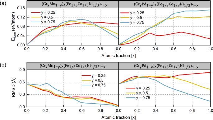
a shows the E_form of FeNiCoCrMn/Pd BCC SPSS systems and b shows the RMSD of FeNiCoCrMn/Pd BCC SPSS systems. The x represents the atomic fraction of CrMn or CrPd elements as the principal component.

Full size image

We calculate several points in Fig. 7 using DFT to validate the predictions of the EFTGAN model. The results of E_form and RMSD predicted by EFTGAN and calculated by DFT are shown in Table 3. The results of predictions exhibit a similar trend to those of the DFT calculations. The MAEs of E_form and RMSD in Table 3 are 0.007 eV/atom and 0.03 Å, respectively. The results show that the EFTGAN model can predict quinary HEAs without significant systematic errors.

The computation of material screening increases exponentially with the dimension of material elements. The EFTGAN model can make the prediction quickly when multiple elemental concentrations change independently. To study the stability of the FCC and BCC systems, the predicted results of E_form and m_s for the ({({{rm{Cr}}}_{0.25}{{rm{Pd}}}_{0.75})}_{0.45}{({{rm{Fe}}}_{{rm{x}}}{{rm{Co}}}_{{rm{y}}}{{rm{Ni}}}_{{rm{z}}})}_{0.55}) system (x + y + z = 1) are shown in Fig. 8. The formation energies E_form at 0 K for the FCC phase and BCC phase are shown in Fig. 8a, b, respectively. We find that E_form for either structure is consistently greater than zero in the composition space, and is relatively small in the region where the concentration of Co is small. However, due to the large mixing entropy of HEAs, the formation free energy at non-zero temperature may be less than zero to form a stable structure. FCC HEAs have good ductility but low strength, while BCC HEAs have excellent strength but insufficient ductility⁴². We have determined the stability of the FCC and BCC phases using the EFTGAN model. In the fully random systems, the S_mix (configuration entropy in case of fully random) takes most important role, we can use S_mix to calculate the stability³⁷. Since the approximately calculated mixing entropy (scriptstyle{{rm{S}}}_{{rm{mix}}}=-{rm{k}}mathop{sum }nolimits_{{rm{i}}=1}^{{rm{n}}}{{rm{c}}}_{{rm{i}}}{{rm{lnc}}}_{{rm{i}}}) is independent of phase, we can determine which phase is relatively stable by the difference in E_form. This result is shown in Fig. 8c, where the blue region represents the composition that the E_form of the FCC phase is lower than that of the BCC phase and the FCC phase is relatively stable, while the red region shows the opposite. We find that the HEA system is more inclined to form the FCC structure at the edge with more Fe-Co or at the edge with more Ni-Co, and is more inclined to form the BCC structure in the remaining region. This may be caused by the larger difference in atomic radius between Fe and Co, which requires more energy in the formation of the more closely packed FCC lattice. The magnetic moments per atom m_s at zero K for the FCC phase and BCC phase are shown in Fig. 8d, e. The BCC phase always has a higher m_s than the FCC phase. The magnetic moment is greater at higher Fe content. Apparently, this is due to the fact that Fe has the largest atomic magnetic moment among of the three Fe, Co and Ni atoms. Based on the results of Fig. 8c, we plot the m_s of the relatively stable phase in Fig. 8f. Since the stabilized BCC phase is located in the high-moment region and the stabilized FCC phase is located in the low-moment region, the magnetic moments of the two phases will have higher maximums or lower minimums compared to those of single-phase systems. We show the free energies (E_form − TS_mix) of high entropy alloys at 400 K and 800 K in Fig. 8g, h. At the temperature of 400 K, the HEAs begin to show a wide range of stable structures in Fig. 8, and when the temperature reaches 800 K, almost all of the HEAs are stable.

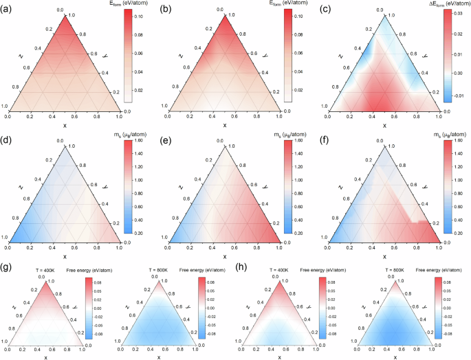
a shows the E_form of the FCC SPSS system, b shows the E_form of the BCC SPSS system and c shows the E_form difference between the FCC phase and the BCC phase for the same composition; d shows the m_s of the FCC system, e shows the m_s of the BCC system and f shows the magnetic moments of relatively stable phases in FCC and BCC systems for the same composition; g shows the free energies of FCC system in 400 K and 800 K, h shows the free energies of BCC system in 400 K and 800 K. The color band to the right of each figures shows the values represented by the colors displayed in each figures.

Full size image

Model extension

The EFTGAN model shows good accuracy on the small data set of HEAs. The objective of this section is to ascertain whether the EFTGAN model is applicable to more complex structures. The model is applied to the inorganic crystal data obtained from the Materials Project (MP)⁴⁴. In order to be consistent with other works, we choose a data set containing 5830 samples to predict the bulk modulus (K_{V RH}) and shear modulus (G_{V RH}). A wide range of inorganic crystals, from simple metals to complex minerals, are included in the data set covering 87 elements and 7 lattice systems. The performances of the models are shown in Table 4. After the data augmentation by the EFTGAN model, the performance is improved over the ECNet model. The EFTGAN model also shows a significant improvement in performance compared to the MEGNet model which is graph-based neural networks²². Seven InfoGANs are trained to generate elemental features for seven lattice systems. The performance of predictions using generated elemental features as inputs is no less than that of the ECNet model. This shows that the EFTGAN model is capable of processing larger samples and more complex structures. The generated elemental features can express complex structural information.

In summary, we have developed a deep learning framework combining elemental convolution and GAN which provides a powerful tool for working with small data set. Through elemental feature extraction, the framework solves the problem of excessive dimensionality of the data generated by the GAN model in material generation. This makes possible for the GAN model to generate elemental features that are responsive to real elemental and structural information. By iterating the generative model with the predictive model, the targets generated by the GAN model are brought closer to the actual values. These ensure the accuracy of the generated data. Therefore, we can use the data generated by the GAN model for data augmentation, which improves the accuracy of the prediction model and solves the problem of insufficient amount of data for HEAs. We also use the idea of transfer learning to address the problem that the predictive ability of the model on the original data is degraded by too much augmented data. In our framework, both generative and predictive models have good generalization capabilities. This facilitates our understanding of the complex relationship in material composition-structure-properties. In addition, our model addresses the complexity of graph neural network inputs by generating elemental features instead of direct computational structures as inputs, enabling fast and accurate large-scale prediction of HEAs. Finally, the trained model is used to predict the formation energies, magnetic moments, and root mean-square displacements of the FeNiCoCrMn/Pd systems. We predict the potential ranges of stable solid solution phases and the trend of magnetic moments as a function of the elemental composition of alloys. These results help to further understand the physics of the HEA systems. The application of our machine learning framework enables the reduction of the requisite train data and satisfies the requirement for the prediction of multi-component materials within a vast compositional space.

Model details and training

In the ECNet model, which is used to extract the elemental features of HEAs, the elemental convolution contains 128 hidden channels, and the multi-layer perceptron contains two feedforward layers with 128 and 64 neurons, respectively. The generator of the InfoGAN model contains transpose convolution layers and a feedforward layer. If the elemental features are considered as different rows of a single channel, the properties of neighboring elements will be convolved together. This will cause non-physical interactions related to the arrangement of the rows of elemental features. Therefore, we consider the elemental features as different channels and the transposed convolution is performed in one dimension. We show two forms of convolution in Fig. S4 of the supplementary material to clarify this problem. The initial inputs to each elemental feature channel are 4-dimensional vectors composed of elemental ratio and 3-dimensional noise. The size of the convolution kernel of each of the three transposed convolutional layers are 1 × 4, and the number of neurons in the feedforward layer is 32. The structures of the discriminator and classifier of the InfoGAN model are similar, containing three convolutional layers with 1 × 3 convolutional kernels and a fully feedforward layer with 32 neurons. In order for the classifier to accurately recognize the elemental composition, we first use the original data to pre-train the classifier, and at this time the generator is also used to generate only data for the known compositions that exist in the original data. After the pre-training, the generator is then trained to generate other composition data. The multi-layer perceptron used for predicting has four hidden feedforward layers containing 32, 16, 8, and 4 neurons, respectively. We first train the perceptron with the generated data and fix the parameters of the first two hidden layers. Then we train the perceptron with the original data.

To evaluate the performance of machine learning models, we follow the standard procedure of dividing the data set into mutually exclusive training, validation, and test sets. The training set is used to train the model, the validation set is used to evaluate when training stops and determine the hyperparameters, and the test set is used to evaluate model performance. Typically, the training, validation and test sets are set to be 80%, 10%, and 10% of the total available data set. We use five-fold cross-validation to test the generalization ability of the model. The data set is divided equally into five parts, one of which is taken at a time to be divided into validation and test sets, and the remaining is used as the training set. We fix the hyperparameters such as learning rate, convolutional kernel size, and batch size, and the performance of the five models in cross-validation are basically the same. Detailed five-fold cross-validation results are shown in Table S1 of the supplementary material, which shows the performance of the EFTGAN models and ECNet models.

DFT calculations

We use the SQS method to model the FCC and BCC SPSS of FeNiCoCrMn/Pd HEAs⁴⁵. The SQS method can provide a structure that is considered as an approximation of the random states. The SQS method randomly places atoms into a standard FCC or BCC lattice to get the structure with the highest entropy, after which we use DFT relaxation to obtain the structure of HEAs. The SQS structures of the binary and ternary alloys used for training were adopted from previous studies,^46,47,48,49 and the data for the quaternary and quintuple alloys are given by our previous work³⁰. For the ternary alloys used to validate the EFTGAN model, we generate their SQS structures by the mcsqs code in the ATAT package⁵⁰. These ternary supercells typically have an atomic number of 20.

All spin-polarized DFT calculations at 0K temperature are performed with the Projector Augmented Wave⁵¹ method which is implemented in the Vienna Ab initio Simulation Package^52,53. The Generalised Gradient Approximation and the Perdew-Burke-Ernzerhof Pseudo-Potential (GGA-PBE) are also used to treat the exchange and correlation energies⁵⁴. We use a 9 × 9 × 9 Monkhorst-Pack mesh⁵⁵ for Brillouin zone integrations. All SQS structures are fully relaxed until all force components are less than 2 meV/Å.