Elastic trapping by acoustoelastically induced transparency

Bound states in the continuum (BICs) exhibit two defining features, namely a frequency within the passband of propagating waves and a wave amplitude of complete zero outside a limited spatial region^1,2. Unlike conventional bound states that exist in bandgaps, BICs are confined modes that coexist with propagating waves in the passband, while leakage is common in passband resonant modes, with the wave amplitude falling. Thus, BICs have emerged as a viable platform for a variety of applications in photonics, especially for molecular sensing/barcoding³ and vortex beam generation⁴, where high-Q-factor modes and radiative modes are desirable at the same frequency.

States in the continuum, often referred to as passbands, cannot be measured across transmission spectra due to their nonradiative nature and vanishing spectral linewidth. Therefore, these states lead to a perfect trapped mode with an infinite Q-factor in principle. In order to visualize the spectrum, a weak radiative nature is indispensable, requiring precise control over an additional perturbation such as structural asymmetry. This results in quasi-BICs, leading to asymmetrical (Fano) lineshapes with wave leakage, particularly in characteristic examples of symmetry-protected BICs.

In the classical wave domains, it is worth noting that BICs are the platform-transparent phenomena, widely studied in the acoustic^{5,6,7,8,9,10,11,12,13}, elastic^14,15,16 and optomechanical^17,18 regimes, following significant cornerstones achieved in the optical regime^{19,20,21,22,23,24,25,26,27,28,29}. Most of the recent research on quasi-BICs has centered on their asymmetric lineshape, which is attributed to the phenomenon of Fano resonance. This effect arises from the interaction between discrete and continuum states, producing a spectrum with an asymmetric profile characterized by a single transmission dip and peak, which originate from destructive and constructive interferences, respectively³⁰.

Considering that Fano resonance is a specific example of quantum interference, we can envisage extending the potential manifestations of BICs by drawing an analogy to another quantum interference. For example, we can expect the observation of quasi-BICs in the form of the electromagnetically induced transparency (EIT)³¹: a more advanced form of the quantum interference that can be achieved using pump-probe spectroscopy where a strong laser probe is utilized to control the behavior of a weak laser pump within a medium. In this context, we directly observe quasi-BICs by means of acoustoelastically induced transparency (AEIT), thus expanding the existing family of BICs that used to be characterized by Fano lineshapes. The AEIT lineshape involves a higher level of complexity, as it requires both direct and indirect couplings to achieve transparency windows in transmission/reflection spectra, resulting in slow vibration driven by highly dispersive behavior. The presented finding is similar to slow light behavior observed in electromagnetically induced transparency (EIT)^22,31,32. Similarly, the plasmon-induced transparency (PIT) process^{33,34,35,36,37}, which illustrates how one aspect of EIT impacts one another, is equally remarkable to observe.

In this study, our strategy for creating an elastic quasi-BIC with AEIT lineshapes is based on multiwave physics domains—elasticity and acoustics—and draws inspiration from the cooling mechanisms in atomic physics^38,39. The proposed design consists of coupled resonators, which are formed by acoustic dual cavities and an elastic bar that interact with each other. This interaction enables the formation of the newly defined AEIT lineshape. These AEIT-oriented quasi-BICs exhibit slow vibration with an ultrahigh-Q-factor and may provide fresh insights into the recently studied Fano lineshape-driven quasi-BICs.

Theoretical and continuum models with coupled resonators

Here we describe the formalism of AEIT for observing coherence effects. In general, the temporal coupled mode theory (TCMT), commonly used to describe optical microring resonators in m-port systems, can be expressed as (dot{{{{bf{a}}}}}=(jPsi -Gamma ){{{bf{a}}}}+{K}^{T}| {s}_{+}left.rightrangle) and (| {s}_{-}left.rightrangle =C| {s}_{+}left.rightrangle +D{{{bf{a}}}}) where a is the n-th resonator amplitude column vector, Ψ is the resonating frequencies in a diagonal matrix, Γ indicates the decaying components, and (| {s}_{+}left.rightrangle) and (| {s}_{-}left.rightrangle) represent the input and output resonating modes through m-th port with the scattering matrix C and coupling matrices K^T and D (see details in ref. ⁴⁰).

In the following, we start by incorporating an additional coupling component κ, which undergoes direct coupling between cavity modes. This incorporation results in a phase shift in the steady state and frequency splitting. Then, we integrate this component into generic TCMT formulae. By considering a two-mode and four-port system (Fig. 1a), the dynamics of the system can be modeled with the following equations:

where a zero-detuning frequency δ_n = ω₀ − ω_n with ω_n = 0 is considered. γ₁ = γ₂ = γ is the decay rate and s_± denotes the amplitude of the incoming and outgoing waves into the cavity. It properly leads to the transmission coefficient (see derivation details in Methods) as

where the relation k ~ ω₀ with the wavenumber k is applied, and d is the distance between two resonators. The system, which consists of dual cavities side-coupled to the waveguide with key parameters (κ, γ), is realized by an elastic continuum bar with two enclosed acoustic cavities shown in Fig. 1b. A more realistic half-sectional configuration is also provided in the zoomed-in image. The interaction between the elastic and acoustic systems is governed by two key parameters, κ and γ, which are associated with the separation distance d between the two acoustic cavities and the volume of the acoustic cavity in the continuum model. The manipulation of these geometric parameters plays a crucial role in shaping the lineshape of the AEIT phenomenon with the field trap. To observe the AEIT phenomenon effectively, it is essential to have large-volume acoustic cavities, ensuring a strong coupling between the cavities and the bar. Thus, we can establish a simplified model that allows control over the single tuning variable d for the purpose of elastic trapping. The end boundaries of two acoustic cavities function as virtual spatial mirrors, activated when the zeroth-order modes of the acoustically local resonance align with those of the elastically local Fabry-Pérot resonance. Notably, the operating principle and corresponding geometry of the virtual mirror effect bear the hallmarks of fixed boundaries, even though they are part of an elastic medium that allows for wave propagation and possesses scale-invariant characteristics (see Supplementary Note 1).

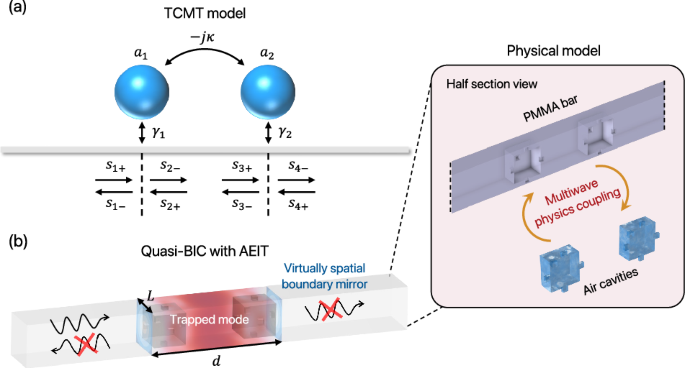
a Schematic of a two-cavity system (cavity mode a) exhibiting direct coupling κ and indirect coupling γ, connected to a waveguide (gray bar) with incoming and outgoing amplitues denoted as s. b Configuration of two acoustic cavities that are coupled to the elastic bar, resulting in a highly confined field trap by a quasi-BIC with AEIT lineshape, making virtual mirror boundaries in the vicinity of acoustic cavities. The entire bar has a dimension of 45 cm × 4.4 cm × 4.4 cm. The length L of the acoustic cavity is 3.33 cm and the side-attached acoustic single supporter has a dimension of 1.11 cm × 0.555 cm × 0.555 cm. The property details of the PMMA elastic bar and the acoustic cavities can be found in “Methods”.

Full size image

Characterization of quasi-BICs by AEIT

Employing a transfer function method⁴¹, we calculate the transmission spectra T = ∣t∣² as a function of frequency and distance d between two acoustic cavities for the three models (Fig. 2a–c). Computational details are provided in Methods. Departing from the acoustoelastic coupled bar illustrated in Fig. 1b, we now introduce two supplementary models—the naked bar and the non-coupled bar—in an effort to investigate quasi-BICs and the impact of enclosed air cavities within the elastic continuum bar. In the case of the naked bar (Fig. 2a), air cavities are filled with the same elastic material as the rest of the bar. Therefore, the elastic naked bar allows waves to propagate in a manner similar to free space, as T remains consistently equal to 1 across all values of d and frequencies in the transmission spectrum. For the non-coupled bar (Fig. 2b), air cavities are present; however, the acoustoelastic coupling is disregarded. In this scenario, the cavity region is treated as an empty space within the elastic bar. The single peak and dip appear (black dashed lines), mainly due to global Fabry-Pérot resonance across the entire structure. Interestingly, in the coupled bar where multiwave physics coupling is active, we observe a vanishing linewidth in the T spectrum at d = 139.521 mm along the orange solid line. This phenomenon indicates a true BIC, where the singular point forms a trapped mode. This mode lacks any sharp spectral features and is, therefore, not measurable (Fig. 2c). In contrast, the neighboring blue and red solid lines represent quasi-BICs with finite linewidths, which are now measurable in the T spectra. The corresponding T spectrum in Fig. 2d, along with its associated d values, confirms that the presence of elastoacoustic coupling is indeed essential in realizing both BIC and quasi-BICs within this system.

A surface plot for T with a color bar indicating the strength for (a) naked bar, (b) non-coupled bar, and c coupled bar. In (c), The presence of a vanishing linewidth, which corresponds to the BIC, is highlighted by the orange dashed line along the frequency and the parameter d. Also, two choices of quasi-BICs are illustrated by blue and red solid lines. d The corresponding T (solid lines) spectra with fixed values in d at the first quasi-BIC (d = 125.331 mm, blue), the BIC (d = 139.521 mm, orange), and the second quasi-BIC (d = 154.01 mm, red). The black dashed line represents that the single cavity is placed with no trapped mode.

Full size image

The signature of the EIT analogy in our acoustoelastic system—two dips and a single peak—is more apparent in the logarithmic transmission (log (T)) (Figs. 3 and 4a). This mechanism is supported by the observation of a large group delay of the transmitted wave, which now results in the formation of quasi-BICs through AEIT. The acoustic cavities, radiant elements in a reflective way, perturb elastic radiation back coherently by behaving as a dipole-like resonator. The elastic bar, on the other hand, functions as a subradiant element that couples indirectly to the acoustic cavities. Together, these well-balanced elements give rise to the AEIT phenomenon and the formation of the quasi-BIC. The energy level landscape depicted in Fig. 3 may provide insight into this characteristic. The presence of κ leads to the splitting of frequencies into acoustically degenerate local resonating states, which is analogous to the dressed states observed in two-photon resonance⁴². These states are excited from the rigid body state (in analogy to the ground state) by the in-plane elastic wave at the left side of the elastic bar. This excitation gives rise to the appearance of two dips in T. Each dip observed corresponds to a total reflection of elastic waves occurring at both the front and back cavities while possessing acoustic traps (Fig. 4a).

The left and right panels represent the first and second quasi-BICs as visualized in Fig. 2c. The acoustically degenerate local resonance gives rise to the acoustic dressed state, which exhibits a single peak (T = 1) in the transmission spectra. In contrast, the elastic dark state is induced by the elastic local Fabry-Pérot resonance, resulting in two dips (T = 0).

Full size image

a (log (T)) across frequencies reveals two dips corresponding to total reflection of elastic waves at the front and back cavities during acoustic resonance. The single peak (shaded region) indicates the elastic trap localized between the cavities. b ϕ at the dips in (log (T)) shows a π phase shift upon reflection at the cavities, while the steep phase transition at the peak represents the elastic trap. c τ_g clearly exhibits large values, indicating a slow vibration mechanism. The TCMT fitting parameters (κ, γ) for the first and second quasi-BICs are (−0.001, 1.7) and (0.001, −1), respectively, demonstrating strong agreement with FEM results.

Full size image

In atomic EIT systems, an external pump beam is commonly employed to stimulate the coupling between energy levels. However, in our AEIT system, the dark state is self-induced by the spatial separation d between the two cavities. The coupling between the radiative and subradiant elements leads to AEIT lineshapes characterized by a single transmission peak and two dips. The position of the single peak, where the trapped mode is formed, can be finely tuned by adjusting the parameter d carefully while maintaining the elastically local Fabry-Pérot state (in analogy to the dark state). The sudden evolution from BIC to AEIT lineshapes and the transition of trapping states are discussed in Supplementary Note 2. The phase shift (phi =arg (t)) at the two dips indicates that the incoming wave undergoes a π phase shift upon total reflection at each acoustic cavity (Fig. 4b). Notably, the opposite evolutions of the relative phases with respect to ω₀ in the first and second quasi-BIC exhibit the origin of anti-symmetric Fano resonances in each AEIT profile. Plus, the steep phase profile observed in the shaded region at the peaks originally signifies the presence of quasi-BICs in (log (T)), which gives rise to the trapped modes. These steep phase transitions provide evidence of slow vibration characterized by large group delays ({tau }_{g}=leftvert dphi (omega )/domega rightvert) (Fig. 4c), which can be compared to the group delay of the naked elastic bar without incorporating acoustic cavities (see Supplementary Note 3). All calculations on (log (T)), ϕ, and τ_g by finite element method (FEM) and TCMT with fitting parameters are well compatible with a good agreement.

Eigenfield distributions and Q-factor calibration in BIC/quasi-BICs

We show the intensity distribution of the elastic eigenfield u and the pressure p in the acoustic cavities to visually illustrate the concept of BIC and quasi-BIC interacting in two different physics domains, namely the acoustoelastic effect (Fig. 5a). Acoustic cavities play the role of dipole-like resonators, and the in-plane vibration mode is indeed confined between the cavities at the peaks (d = 125.331 mm, first panel, and d = 154.01 mm, third panel) in the quasi-BICs and at the singular point (d = 139.521 mm, second panel) in the BIC. Moreover, the normalized absolute displacement field ∣u∣ supports the signature of BIC and quasi-BICs (Fig. 5b). The value completely drops to zero decoupling from the radiational elastic waveguide is represented by the BIC (orange line), and small leakage in the vicinity of the cavities represents quasi-BICs (blue and red lines). The end-to-end region between cavities makes a virtual mirror effect from the destructive interference via the acoustoelastic coupling. The Q-factor is also estimated at the corresponding d (Fig. 5c). Based on the elaborated position for the BIC (orange dashed line), a smooth lowering of the Q-factor can be obtained by varying d to have quasi-BICs (blue and red dashed lines). Since we tune the spatial dimension between acoustic cavities for BIC and quasi-BICs, the Purcell factor F_p^43,44 may be essential to investigate for making a miniaturized form factor, which is proportional to Q/V where V is the mode volume expressed as (Vpropto {int}_{Omega }| u{| }^{2},dOmega /max (| u{| }^{2})) where Ω is the volume in elastic domain between two acoustic cavities. The increase of F_p allows us to have highly efficient wave confinement when compared to reduced mode volume. Through this consideration, we obtain the corresponding F_p; 4.8366 × 10⁹ at d = 125.331 mm, 1.0538 × 10¹⁵ at d = 139.521 mm, and 7.0585 × 10⁹ at d = 154.01 mm, achieving the tunability of the Purcell factor by around six orders of magnitude.

a Eigenfield distributions of ∣u∣² and p in the BIC and quasi-BICs visualized through quarter-section views. b ∣u∣ along x-axis. The region (50 mm long) beyond 200 mm is designated for the implementation of the perfectly matched layer (PML). The acoustoelastic coupling gives rise to the virtual mirror effect located at the black dashed line, indicating the end-to-end distance between acoustic cavities. The BIC (orange) effectively decouples from the surrounding waveguide, resulting in a complete suppression of energy leakage. In the case of quasi-BICs (blue and red), the trapped modes are not perfectly isolated from the surrounding waveguide, and there is a small amount of energy leaking out. This results in the lowering Q-factors in (c).

Full size image

Experimental validation

We conduct experiments to investigate the existence of quasi-BICs with AEIT by using a PMMA elastic specimen integrated with acoustic cavities while keeping the same geometric configuration as in the previous analysis (Fig. 6a). The openings of the acoustic cavity are sealed off from the surrounding air (ambient pressure) using vacuum bag sealant tapes. In practical situations, we have a finite bar instead of an infinite one with perfect absorbing conditions probed by the transfer function method, and therefore, we measure the acceleration using sensors attached to the right-end boundary and the source part. For excitation, we use an electromagnetic shaker to produce an in-plane elastic source (see “Methods” for experimental details). We conduct measurements of the acceleration ratio, a_out/a_in, along the x-axis using the quasi-BIC sample for d = 125.331 mm, where a_out and a_in denote the out and input accelerations. It is worth noting that intrinsic material loss is inevitable, and we account for this by introducing complex-valued losses as E* = E_e(1 + jη) and c* = c_a(1 + jζ) for elastic modulus and sound speed of air. We determine elastic loss η by measuring the Q-factor (see the loss measure in Supplementary Note 4), and the acoustic loss ζ is also obtained by fitting and comparing experimental and numerical data. Due to the presence of material loss, the experimentally captured acceleration no longer fits the AEIT lineshape and instead resembles the Fano lineshape, with the single dip disappearing. Despite this, it is essential to point out that the trapped mechanism can still be witnessed at the peak (Fig. 6b). The global Fabry-Pérot state, which results from the entire elastic bar being inside the free spectral range, is responsible for the apparent sloping trend in the observation (see Supplementary Note 5). Incorporating material loss into the eigenanalysis allows for recalculation of the Q-factor and Purcell factor as 433.36 and 2.1708 × 10⁷, which still remains robust due to quasi-BICs with AEIT lineshapes. The Q-factor of 404.274 is also determined using the FWHM method, based on the experimental data in Fig. 6b. We expect that the design strategy presented in this study can be applied to systems of various sizes and target frequency ranges without loss of generality. Moreover, it is applicable to any form of materials in the elastic domain, especially denser materials that work at shorter wavelengths, where material loss is typically lowering. This flexibility enables the implementation of our design approach across a wide range of scenarios, allowing for customization based on specific system requirements without losing functional integrity.

a Illustration of the experimental setup including a fabricated elastic bar with acoustic cavities. b a_out/a_in obtained by FEM (blue solid line) and experiment (colored circles) results including the elastic loss η = 0.072 and acoustic loss ζ = 0.0011. The peaks (arrows) indicate the elastic trapping states.

Full size image

We provide insights into the acoustoelastic interaction within a coupled resonator system, highlighting the potential to manipulate quasi-BICs through acoustoelastically induced transparency (AEIT). This phenomenon mirrors the electromagnetically induced transparency (EIT) observed in atomic systems, thereby enriching our understanding of BICs and expanding their observations in acoustics and photonics. By harnessing multiwave physics across domains, namely acoustoelasticity, the proposed system—composed of dual acoustic cavities embedded in an elastic medium—generates slow vibration phenomena similar to slow light effects found in optical systems. The exploration of AEIT in acoustoelastic systems marks a notable step forward in our ability to control wave propagation in complex media, paving the way for the design of highly tunable and responsive devices. These findings broaden the catalog of existing BIC phenomena, extending beyond Fano-driven lineshapes to now include AEIT lineshapes, while enhancing our capability to engineer high-performance devices tailored to specific technological needs. The proposed strategy may offer broad potential across various areas, such as precision sensing, advanced lasing and screening techniques, and energy storage systems. In particular, we anticipate exciting possibilities for developing novel technologies that leverage acoustoelastic interactions, enabling next-generation real-time material/defect characterization, elastic wave spectroscopy, structural health monitoring, and self-powered sensors for IoT devices and wearable electronics via piezoelectric energy harvesting—applications where ultrahigh-Q-factor modes are in demand.

Materials and sample fabrication

The proposed specimen was based on the photo-polymer UV resin and 3D-printed with the following properties: E_e = 2.56 GPa (Young’s modulus), ν = 0.35 (Poisson’s ratio), and ρ = 1127 kg/m³ (density). By attaching the vacuum bag sealant tapes, the internal cavity was isolated from the background and was determined by c_a = 343 m/s (speed of sound) and 1.2 kg/m³ (density).

Numerical simulation

Throughout this work, the three-dimensional full-wave simulations were conducted with a commercial finite-element solver software—COMSOL MULTIPHYSICS. The structural mechanics and acoustics modules were used to verify the BIC/quasi-BICs by acoustic-structure interaction. Measurements of the T spectra were conducted using the transfer function method⁴¹ in Fig. 2, and T values were properly bounded in [0, 1] with in-plane (longitudinal) mode excitation, indicating that other modes are not present in our proposed structure. The frequency domain analysis was used for calculations of T spectra, where the in-plane elastic source and the PML were imposed at the left and right end boundaries while tuning the geometric parameter d. In the eigenmode analysis, field distributions were visualized, and Q-factors and F_p were calculated.

Derivation details on t and T

In the set of ordinary differential equations (Eq. (1)) by TCMT, we incorporate relations:

where γ₁ = γ₂ = γ and s₄₊ = 0 in which the incoming wave propagates from the left port, and the assumptions of a ~ e^jωt and k ~ ω₀ have been considered. Accordingly, we have

By defining t = s₄₋/s₁₊, we thus arrive at Eq. (2).

The transmission spectrum can also be derived by T = ∣t∣² = t ⋅ t* and the corresponding expression is written as

where (A=-{gamma }^{2}+2jgamma kappa {e}^{-j{omega }_{0}d}+({kappa }^{2}-{(jgamma -{omega }_{0})}^{2}){e}^{-2j{omega }_{0}d}) and * indicates the complex conjugate.

Also, the phase (phi =arg (t)) and the group delay τ_g = ∣dϕ(ω)/dω∣ are numerically computed to characterize slow vibration. During the computation of τ_g, it is essential to exclude the data points corresponding to the occurrence of a discontinuity. These discontinuities manifest when two reflections take place, one at the front cavity and the other at the back cavity.

For the case of the single cavity coupled to the waveguide as in Fig. 2d, the TCMT equation is written as

With assumptions of a ~ e^jωt and s₂₊ = 0, it gives rise to

which further derives into t = s₂₋/s₁₊ and the transmission spectra is as follows:

This formula confirms that the trapped mode, characterized by a peak, is absent in comparison to the coupled system involving two cavities (Fig. 7, solid line).

The solid line indicates a model with no side coupling that provides a symmetric profile. On the other hand, the dashed line indicates a model with side coupling, resulting in an asymmetric profile.

Full size image

Similarly, we further consider the side coupling since the proposed model has different symmetries along x-axis and y– and z-axes. The TCMT equations would be

where β is the side coupling and ϕ is the phase. The additional channel 3, which can be thought of as s₃₊ = ∑_i=1s_i+ running over the set i = ( ± y, ± z), is implemented for side coupling effect in such a symmetry. By incorporating relations s₃₊ = s₁₊e^jϕ and ({s}_{2-}=({s}_{1+}+{s}_{3+}-a(sqrt{gamma }+sqrt{beta }))/2), we have the T spectra as

where (B=j(beta -sqrt{gamma beta })+{e}^{-jphi }(j(gamma -sqrt{gamma beta })+omega -{omega }_{0})+omega -{omega }_{0}). This aspect is not taken into account in the calculation of AEIT lineshapes in the main text, as it primarily influences the degree of asymmetry, particularly in the tail drops of T spectra at higher frequencies of interest. This gives rise to an asymmetric profile (Fig. 7, dashed line) which is similar to the data obtained from the FEM result of the 3D single cavity model in Fig. 2d.

Experimental details

The experimental flow is as follows: the vibration is induced by amplifying the source signal from a function generator (Agilent 33220A) using a linear power amplifier (LDS LPA600) and transmitting it to an electromagnetic shaker (LDS vibrator V406). To facilitate easy tracing of the vibration, the trigger source of the function generator is connected to an oscilloscope (Keysight DSOX1204A). The source condition is employed to construct a stretched pulse defined by (A(t)={A}_{0}sin left[2pi left({f}_{i}t+frac{({f}_{t}-{f}_{i})}{2P}{t}^{2}right)right]) where A₀ = 1 and P = 10 s (period). The frequency range of interest is defined as [4700, 5200] Hz, with f_i representing the initial frequency and f_t representing the terminal frequency. The time duration considered is from t = 0 to t = 10 s. By applying the fast Fourier transform (FFT) to the data, the amplitude of the FFT is achieved so that a consistent response can be obtained from the source signal in the frequency range of interest. The accelerations, both input and output, are measured using two accelerometers (PCB 356B21). These accelerometers are attached to the bottom of the aluminum plate and the top of the specimen, respectively. The voltage outputs from the accelerometers are then routed to the oscilloscope via a signal conditioner (PCB 482C05). The purpose of the signal conditioner is to process and adjust the voltage signals from the accelerometers, ensuring reliable measurements. Once the signal is captured on the oscilloscope, it is transferred to a laptop. On the laptop, the recorded signal undergoes the FFT algorithm, which enables frequency analysis. The FFT algorithm converts the time-domain signal into its frequency-domain representation, allowing for the examination of the spectral characteristics of the signal.