Energy landscape of conformational changes for a single unmodified protein

Introduction
In the physiological environment, proteins exist not as single rigid structures, but as dynamic entities sampling many conformations across a free-energy landscape. At the most basic level, the free-energy landscape is a graph of energy across a reaction coordinate that underlies the thermodynamics, and at the single-molecule level, the molecular biophysics. Conformational dynamics are a common example of trajectories on the energy landscape, largely responsible for protein function. To observe these dynamics, single-molecule approaches are favoured because they do not require synchronisation and naturally allow for observing heterogeneity1.
Common approaches to single molecule investigations of proteins employ labels (e.g., in Förster resonance energy transfer)2,3,4 or tethers (e.g., in force-measurement techniques)5,6,7,8,9,10,11. While these have been highly successful, they are not without challenges in terms of observation time and energy scale (e.g., pulling measurements apply forces that completely unravel the protein). These techniques also require the introduction of a label or tether (with additional steps, more hardware, and perhaps modifying the intrinsic function of the protein12,13,14,15,16,17,18,19). Therefore, approaches that can directly observe unmodified protein conformation dynamics at the single molecule level are desired. While many approaches are emerging to observe unmodified proteins (label-free, tether-free)20,21,22,23,24,25,26,27,28,29,30,31, so far the conformational dynamics of a single unmodified protein remain largely unexplored.
Nanoaperture optical tweezers (NOTs) have been employed by many groups to observe biomolecules and nanoparticles at the single molecule level without the need for any modification21,24,32,33,34,35,36,37,38,39,40,41,42,43,44,45,46,47. The first work to demonstrate the trapping of a single protein with NOTs used Bovine Serum Albumin (BSA) as a model system34. In that work, the conformational changes of BSA were seen by changes in the optical transmission of the trapping laser beam through the nanoaperture, where transitions from the normal to fast form of the protein resulted in an increase in transmission. This was confirmed by lowering the pH and forcing the BSA into the fast form so that only the larger transmission state was observed. However, quantifying the observed dynamics and using them to determine the energy landscape was not shown in that work. A direct measurement of a single protein’s energy landscape can lead to a better understanding of thermodynamic properties, allostery, intrinsically disordered proteins and prion diseases, to name a few examples.
Here we show the connection between the probability density function (PDF) of the trapping laser’s scattering and the energy landscape along the protein conformation reaction coordinate. We produce the free-energy landscape governing normal (N), fast (F), and expanded (E) conformations of BSA, mapping out changes in the landscape with temperature. We quantify the thermodynamics of these transitions, finding the entropy change associated with a transition and using a Markov model with Kramers’ transition rate probabilities to capture the observed dynamics. We also observe dimer formation in the trap (directly seen when a second BSA enters the trap). We show that the dimer formation has a stabilising effect, suppressing F and E forms, while we quantify the open (O) and closed (C) hinge transitions of the dimer.
Our work follows a large body of literature on BSA. BSA is a 66 kDa water-soluble monomeric protein that is the most abundant protein in blood (40-50 mg/mL). Its structure is well studied and the conformational changes are largely explained by changes in the disulphide bridges of the Cys residues48,49,50,51,52. Adjacent Cys residues are unable to form disulphide bridges because the highly favoured trans-peptide bond during folding prevents the sulfhydryl groups from being close enough to bond. Thus, the adjacent Cys residues must bridge to Cys residues further away. Three domains emerge where the polypeptide backbone is joined by the double-Cys bridge (domains I, II, II). These three domains are similar, formed by six α-helices arranged in a heart shape with 17 disulphide bond linkages stabilising the domains and one sulfhydryl group (Cys-34, domain I, hydrophobic pocket). Each domain is composed of two subdomains (A and B). BSA has dimensions 80 × 80 × 40 Å3 and is composed of 583 amino acid residues. Key to the function of BSA are the hydrophobic pockets that are not exposed to water in the N form, but are exposed in the F and E forms. At neutral pH, the disulphide bridges are buried in the protein and not exposed to solvent.
BSA conformations have typically been probed using pH changes53,54,55,56,57 and temperature changes58,59,60,61. These conformational changes are reversible (provided the temperature is below 55 °C62,63). At room temperature and neutral pH, BSA exists in the N-state (heart shape), and at pH 3.5, it undergoes a conformational transformation into a more linear shape F-state. Three independent folded conformations have been observed by smFRET and differential scanning calorimetry64,65, with the E state being the most expanded. To remain consistent in the terminology used with pH experiments, we define the three states observed in our experiments as N, F, and E, indicating native, expanded due to domain III opening, and maximally expanded due to domain I and III opening.
Results
Experimental configuration
Details of the experiment are presented in the Methods section. Briefly, a simplified schematic of the optical tweezers is shown in Fig. 1a. A schematic of the microwell, an electron microscope image of a double nanohole (DNH), and an image of a DNH on the camera is seen in the expanded view. Simulations of the electric field enhancement and thermal distribution with a 980 nm incident laser are shown in Fig. 1b, c. The local temperature increase due to heating from an incident laser on a nanoaperture has been studied in multiple works42,66,67,68, with values reported from 0.6 K/mW to 3.6 K/mW. We performed COMSOL simulations of the local heating and estimated 0.58 K/mW of laser power as defined after the microscope objective (see Fig. SI-1a, b) In past experiments on a nominally identical setup, we used ratiometric analysis of upconverter emission to determine the local temperature changes with laser power, and found 0.64 K/mW was the heating68. The local temperature at the protein was varied by changing the trapping laser power.

a Simplified microscope diagram. Laser passes through a linear polarizer and half-waveplate to control polarisation orientation and a beam expander to fill the objective. A 100 × 1.25 NA oil immersion objective is incident on the sample and transmitted light is collected by a 10 × 0.25 NA objective and recorded on an avalanche photodiode (APD). Inset: Schematic of microwell used for trapping solution and SEM and camera image of a DNH used in experiments. Camera image is under focused to highlight the oval shape of the DNH and represent the focus state during trapping. b Electric field and (c) thermal distribution simulated by COMSOL Multiphysics for a DNH in aqueous using incident 980 nm laser with 1 mW power and beam diameter of 1 μm.
Protein dynamics
Conformational changes of a protein alter the structure, and thus the polarizability69. This changes the transmission through the DNH. As a control experiment, Fig. 2a shows a trapping event of a 30 nm diameter polystyrene nanoparticle that does not change conformation upon trapping at different temperatures. We expect that the trapping position for PS nanoparticles is the same as BSA because of the larger sized gap used. The transmission is stable for all temperatures as there is no structural rearrangement, nor is there evidence that the translational motion in the trap would result in discrete levels of the signal that we present next for conformational changes. Since the temperature increase is attained by increasing the laser power, the signal to noise ratio also increases (signal increases linearly with laser power and noise as the square root, since we are in the shot-noise limited regime).
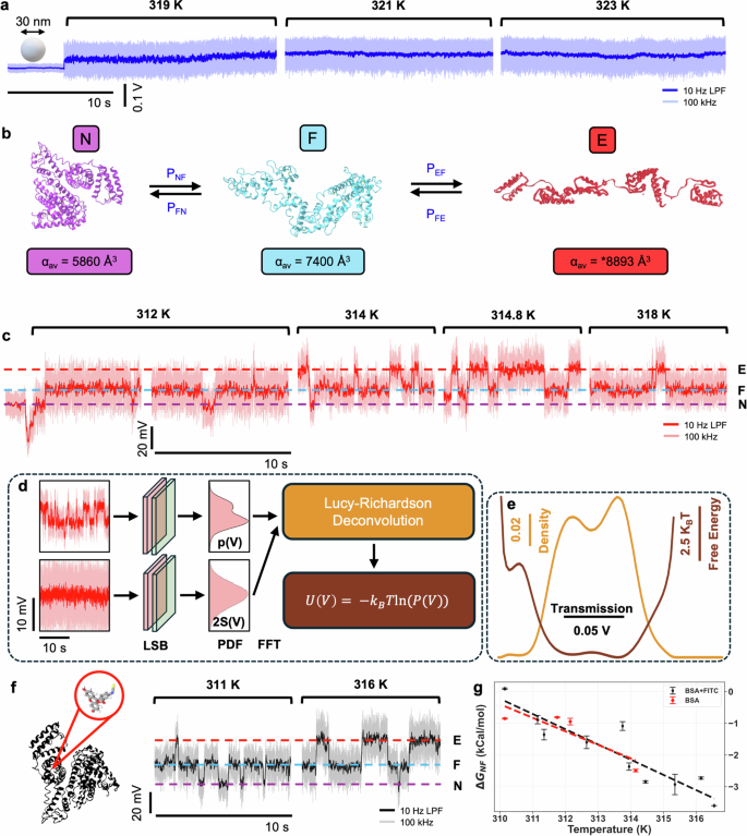
a Transmission through the DNH at different temperatures for a 30 nm polystyrene nanoparticle trap. Dark blue indicates data filtered with a 10 Hz low-pass filter, light blue indicates data sampled at 100 kHz. b Reaction mechanism diagram for the forward and reverse conformational changes of N ↔ F and F ↔ E and the corresponding average molecular polarizabilities. Proteins visualised using PDB: 3V03 for the N-state and PDB: “F isoform of BSA at pH 3.549” for the F-state. No 3D structure is available for the E-state, illustration is traced past work77. Polarizability estimated from experimental data. c Transmission through the DNH measured at different temperatures for a single unlabelled BSA trap. Dark red indicates data filtered with a 10 Hz low-pass filter, light red is raw data at 100 kHz. d Deconvolution of transmission probability density function (100 bins, 100 kHz sampling rate) and PSF to obtain the energy landscape. LSB least significant bit dithering, PDF probability density function. e Energy landscape and probability density function after deconvolution for unlabelled BSA at 314 K. f Transmission through the DNH measured at different temperatures for a single FITC labelled BSA trap. Black indicates data filtered with 10 Hz low-pass filter, grey is raw data at 100 kHz. g Change in Gibbs free energy for unlabelled and labelled BSA, obtained from the energy landscape at different temperatures.
Figure 2b shows the N- and F-state of monomeric BSA with average molecular polarizabilities calculated to be 5860 Å3 (PDB: 3V03) and 7400 Å3 (PDB: F isoform of BSA at pH 3.549) using an atomistic model of the protein69 and visualised using iCn3D70. There is no PDB molecular structure available for the E-state; however, the polarizability can be estimated at 8893 Å3, as extrapolated from the root mean square deviation of the signal for the laser, N, and F states (see Supplementary Information Fig SI-3 and Table SI-1).
Conformational changes of a single BSA protein are easily identified as changes in transmission through the DNH. Figure 2c shows the effect of temperature increase on the dynamics of a single BSA. The dip in transmission signal is seen in all trapping events for both proteins and polystyrene nanoparticles, this is due to the scattering phase change around the aperture leading to destructive interference during the initial stage of trapping. The protein is initially trapped in the N-state, as expected, and quickly transitions to the F-state. The transitions at 312 K mostly fluctuate between F- and N-, with a rare E- occurrence. As the temperature is increased, the rate of N ↔ F and F ↔ E transitions shifts to favour the more expanded form.
The energy landscape of these conformational changes can be obtained from the PDF, a binned histogram of the APD voltage recorded for an extended time-window. For force-measurement approaches, the deconvolution of a point spread function (PSF) has been widely investigated as the tethers are fluctuating separately from the conformational dynamics of the protein9. Here, the translational or rotational motion of the protein will give fluctuations to the signal that are distinct from conformational changes. These fluctuations (and other factors such as noise) give a PSF to the signal that should be deconvolved to extract the true PDF associated with the conformational changes and from this, the energy landscape. The energy landscape and PSF are determined from the raw data sampled at 100 kHz. Filtering of the data necessarily constrains the trapping signal into the region of the energy landscape minima, artificially changing the extracted biophysical parameters, and so this is not done when producing the energy landscape.
For rigid structures, the distribution from translational motion is well-fit by a Gaussian, with FWHM linearly proportional to the protein molecular weight, as found previously for multiple proteins71. Using this information, we can estimate a PSF, C(V), for our BSA measurements to have a standard deviation of 13.4 mV, which we can determine from calibration curves like in past works71, but here we get it from the dimer due to the enhanced conformational stability allowing for longer observation without a transition. We investigated the impact of small variations on the robustness of this PSF and found little variation within 1.2 mV deviations.
The PDF of the raw transmission data, p(V), was deconvolved with the Gaussian PSF using the iterative Lucy-Richardson algorithm to uncover the energy landscape P(V):
where k is the iteration number, ⊗ denotes convolution, and ({*}) denotes complex conjugate, with P(V)(1) = p(V). P(V) = P(V)M, with M = 51 being the total number of iterations to achieve convergence.
The energy landscape was thus obtained by the following equation:
where kB is the Boltzmann constant and T is the temperature. A schematic overview of this process is shown in Fig. 2d and the resulting PDF and energy landscape of BSA at 314 K is shown in Fig. 2e.
We repeated the measurement with fluorescein isothiocyanate (FITC) labelled BSA to see if different results would be obtained for the labelled form. FITC binds to site II of BSA, filling an empty hydrophobic site of domain III, noting the FITC itself is also hydrophobic. A schematic of FITC-BSA and a transmission time trace at different temperatures is shown in Fig. 2f. The change in Gibbs free energy for both labelled and unlabelled data is shown in Fig. 2g, demonstrating a temperature dependence on the spontaneity of the conformational changes and equilibria of states.
The energy landscape evolution with temperature is shown in Fig. 3a. The energy minima shows an evolution towards E and F states, and away from N state as the temperature increases, as noted by changes in the relative Gibbs free energies of these minima. Quantitative values are obtained from the landscape by measuring free energy differences between states and the curvatures of the wells and barriers, as shown in Fig. 3b. Examples of well and barrier curvatures for two temperatures, 310 K and 314 K are shown in Fig. 3c.
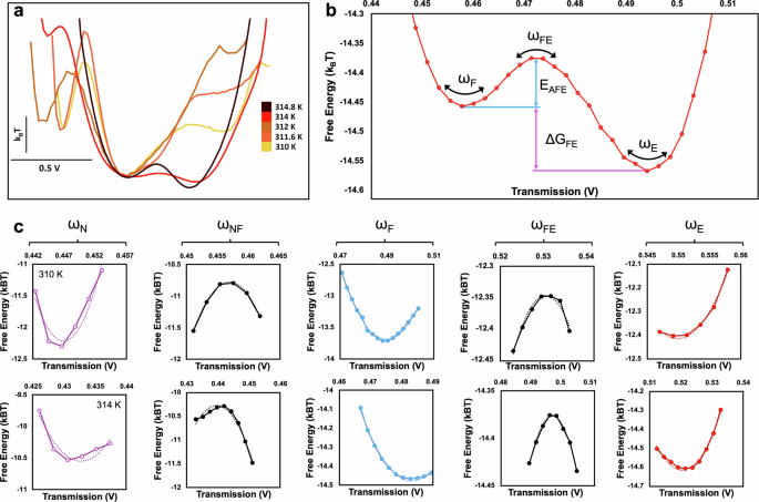
a Energy landscapes for trapping events at increasing temperatures. b Example of quantitative values obtained from the energy landscape, where ω is the curvature, EAFE is the activation energy for the FE transition, and ΔGFE is the change in Gibb’s free energy of the FE transition. c Curvatures from the energy landscape fit to a second order polynomial at 310 K and 314 K.
The thermodynamic equilibrium constant, K, is the quotient of the activity of the reaction and is dependent only on temperature, T. A large K value indicates a highly favoured product, or in this case, a favoured conformation. This follows the equation:
where ΔG is the change in Gibbs free energy and R is the gas constant. We calculate Keq using the minima in the energy landscape, with more detail found in the Methods section.
We define two pathways in this work, the N ↔ F and F ↔ E. To verify the efficacy of the deconvolution in retrieving accurate biophysical parameters, two other analyses were performed for comparison: Markov chain simulations and residence time ratio analysis. In the Markov chain simulation, the probabilities of each pathway and the transition matrix were defined as in Fig. 4a. Further to this, Kramers’ theory in the viscous damping limit describes the forward flux of the reaction as follows72:
where ωN is the curvature of the N energy minimum, ωNF, is the curvature of the N-F barrier, ζ is the friction coefficient, and EANF the activation energy going from N to F. The curvatures of the N, F, and E minima as well as the barrier curvatures were obtained directly from the energy landscapes (see Supplementary Information Fig. SI-4). Four probabilities are then defined as:
and the individual proportionality constants are obtained via the PNF proportionality constant and the ratio of curvatures for the barriers and wells:
In the residence time analysis, the thermodynamic equilibrium constant was obtained from the ratio of the total duration in each state. Namely, ({K}_{NF}=frac{{tau }_{F}}{{tau }_{N}}) and ({K}_{FE}=frac{{tau }_{E}}{{tau }_{F}}).
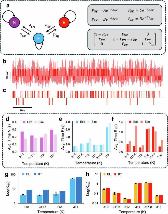
a Markov chain representation of conformations and associated probabilities and transition matrix. b Time series signal of conformational changes at 310 K, raw data in light red, identified states in dark red. c Markov chain simulation of trapping signal using values obtained from energy landscapes. d Average residence time of the N state over a range of temperatures measured from experiments and simulations. e Average residence time of the F state over a range of temperatures measured from experiments and simulations. f Average residence time of the E state over a range of temperatures measured from experiments and simulations. g Comparison of thermodynamic equilibrium constant for the N ↔ F pathway. Values obtained via energy landscape (EL) and residence times (RT). h Comparison of thermodynamic equilibrium constant for the F ↔ E pathway. Values obtained via energy landscape (EL) and residence times (RT).
The segments of energy landscapes used for curvature measurements are shown in the Supplementary Information (Fig. SI-4). The proportionality constant A was optimised using an unconstrained nonlinear optimisation, given the experimental average residence times as the goal. This is the only free parameter of the model. Simulations were run to achieve a 1000 s time series.
The activation energy is obtained from the full time series data (example shown in Fig. 4b). A k-Means state recognition algorithm was used to find the experimental state switching, also shown in part b. Figure 4c shows 80 s of the corresponding Markov simulation using the activation energies and change in Gibbs free energy from the experimental energy landscape. A comparison of the average residence times for the N, F, and E-state is shown in Fig. 4d–f. After verifying the deconvolution result, the thermodynamic equilibrium constant obtained via the energy landscape was compared with kinetic analysis using the full residence time ratios, seen in Fig. 4g, h.
Discussion
Through a deconvolution procedure of the time-averaged data, we have presented the energy landscape of monomeric BSA for various temperatures (see Supplementary Information Fig. SI-5). We then reconnected this with the kinetics by using a Markov model with Kramers’ theory transition rates. In this current study, the PSF was determined using a stable version of the same protein; however, in the future, a calibration curve can be obtained, allowing for the extraction of a PSF for any intermediate protein a priori. The PSF arises from the translational and rotational motion of the protein in the trap, and this is measured by the RMSD and the corner frequency in each state. We found negligible (within 6%) changes in RMSD values between each state, implying that the PSF is approximately state independent. Thus we can use a fixed PSF for conformational changes in a single protein, but the dimer retains the linear proportionality to molecular weight for the PSF. Good qualitative agreement was seen between the Markov model and the observe kinetic data. Quantitatively, the average time from the Markov model agreed well with average residence times from the k-means state recognition. There is a notable exception of the E state for T = 311.6 K, where the energy landscape of this state does not have a pronounced barrier (see Supplementary Information Fig. SI-5) and so perhaps it was not appropriate to apply the Kramers’ theory for that particular case. The main point of the Markov model is to show that we can use Kramers’ theory to explain the underlying biophysics of the conformational changes, i.e., the time domain data. In adopting a viscous damping Kramers model, only a single free parameter exists. While there was one free parameter for fitting the Kramers’ theory for each temperature, these could be further constrained by Eq. (3) from the curvature of the minima and barriers, assuming the viscous damping is only weakly temperature dependent. Indeed, if we divide the fitting parameter by ωNωNF, the value is almost the same (to within 27%) over the different temperatures tested. So, all the time domain dynamics are represented from energy minima and maxima curvatures in the energy landscape. We believe, therefore, that this is the essential information to explain the biophysics of these conformational changes.
The extracted energy landscape was used to provide the equilibrium constants through Eq. (3), and this agreed quantitatively with the ratio of the residence times from the experimental data. This shows accuracy of the deconvolution in producing changes in Gibbs free energy state minima. We showed the deconvolution robustness by attempting slightly different PSF widths, as shown with the error bars. It is also noted that the different states could have different PSFs, and this could explain some of the differences seen between the modelling and the experiments.
While we have extracted the energy landscapes and related Gibbs free energy values, we can consider what these say about the changes in enthalpy and entropy when going between states. The change in Gibbs free energy is related to the change in enthalpy (ΔH) and change in entropy (ΔS) of the protein from the following equation:
For the N to F transition, we observed that change in Gibbs free energy is almost linearly dependent on temperature. This suggests that it is mainly an entropic variation between the different temperatures. Since the entropy is defined by the available degrees of freedom in each state, we expect that S will not change with temperature, but the entropic contribution TΔS will vary linearly with temperature, as expressed in Eq. (7). Using this relation, we found for unlabelled BSA ΔG of 130 ± 55 − 0.43T ± 0.18 kCal/mol, while FITC labelled BSA gave 150 ± 20 − 0.48T ± 0.07 kCal/mol. We have not found any reports of conformational entropy changes for BSA for the N-F transition for 3 states; however, one work reported for only two states and obtained entropy and enthalpy change values in the same order of magnitude as we find here58. For the F to E transition, a simple linear temperature dependence was not observed; indeed, there is a minima in the change of Gibbs free energy with temperature (see Supplementary Information Fig. SI-6) that requires further theoretical support. Also, labelled and unlabelled BSA showed similar but not identical behaviour with temperature changes (see Supplementary Information). Repeatability is shown with good agreement of Gibbs free energy values with measurements over multiple days and DNHs.
The laser power changes the optical force, but the force acts to keep the BSA in the potential minima, where the net force is zero. Therefore, to first approximation, the force changes do not play a role in conformational changes; however, higher order effects, like electrostriction, may have some contribution. Due to the ergodic nature of our observations, electrostriction is expected to not be dominant—the protein transitions between states at all temperatures observed and is not forced into a single particular state.
There is often question of whether trapping is a single protein or an aggregate: using video and photodiode analysis, we showed that the initial trap is of a monomeric protein that forms a dimer when a second protein enters the trap (see Supplementary Information Fig. SI-2 and SI-7). The dynamics found once the dimer was formed in the trap when a second monomer entered matched the observed behaviour seen when a dimer was trapped as a whole. There is a transition from monomer to dimer after a second monomer is trapped. We did not observe the F and E states for the dimer. Previous literature has reported that the large stabilisation energy of dimers comes from intersubunit interactions and is substantially greater than monomeric forms73.
The dimer transitions show a typical two-state system: the closed state of the dimer is the natural formation where the two heart shapes are compact and an open state that is more extended and hence has larger polarizability. We have only found structural data for the compact dimer state, from which the polarizability values were calculated (see Supplementary Information). Calculated and extrapolated values for the polarizabilities are shown in Table SI-1 and Fig SI-3a, b.
We have previously shown the ability to track proteins prior to them entering the trap74. In the present case, we were able to use this capability to confirm that a second BSA molecule was entering the trap after one was already trapped (see Supplementary Information). Once trapped, we could also use the camera to record the changes in the conformation of the protein in the trap (see Supplementary Information Fig. SI-8), which shows that we will be able to perform the entire measurement in the reflection geometry in the future75. This would allow easier integration of microfluidics and external heat control as there would be no concern about the condenser lens path.
In this work, we have used the time dynamics of trapped monomeric and dimeric BSA to uncover the energy landscape of the protein undergoing conformational changes. We used a Markov model with viscous Kramers’ theory to model the observed dynamics from the extracted energy landscape, showing good agreement with the actual observations. We quantified changes in Gibbs free energy between the N, F and E states of BSA, and found changes in enthalpy and entropy between the N and F states to be 132 kcal/mol and 0.43 kcal/mol for unlabelled BSA, and slightly larger values were found for FITC labelled BSA, showing that the impact of labelling is not significant within the precision of this measurement. The F to E transition showed more complicated behaviour. We also observed formation of a dimer in the trap, and found that not only did the dimer exhibit a two state transition, but it also appeared to be stabilised against transitions to the F and E states for each of the subunits. In the future, looking at a fully cross linked version of a protein with known conformational changes could be used to verify specific conformations identified during trapping.
This technique is most interesting to uncover the energy landscape and related biophysics of single proteins because it does not require any modifications to the protein being studied—neither labelling nor tethering. Not only does it make the approach easy to use and useful for assessing the impact of labels, but it also opens the door to studying proteins that are challenging to label reliably, such as intrinsically disordered proteins.
Methods
Colloidal lithography of double nanoholes
DNHs were fabricated using a modified approach from past works76. Standard microscope slides (Fisherbrand 12-550C, 75 × 50 × 1.0 mm3) were cut into thirds using a diamond scribe, cleaned by sonicating in ethanol for ten minutes, and dried under nitrogen. A solution was made of 20 μL of 300 nm polystyrene beads (Alpha Nanotech) and 1 mL of ethanol. Using 10 μL of the polystyrene-ethanol solution, a zig-zag pattern was deposited on the microscope slides and left overnight. Once the ethanol evaporated, the square slides were put in an oxygen plasma machine (Harrick PDC) for 170 s. To ensure reproducibility of aperture size and shape, the slides were etched individually in the same location to ensure consistent plasma coverage. The coated slides were then coated with 7 nm of titanium and 70 nm of gold using a sputter deposition system (Mantis QUBE). Polystyrene was removed from the metal by sonicating upside down in ethanol for 7 min. No surface passivation was used, although we previously investigated the impact of passivation with mPEG-thiol on the same BSA-trapping system and it did not show discernibly different results34.
Trapping solution
A 24 × 60-1 microscope cover glass (Globe Scientific Inc.) was cleaned using isopropyl alcohol and dried under nitrogen. An image spacer (Grace Bio-Labs GBL-654008-100EA) was placed in the centre of the coverslip and 9.37 μL of the solution was pipetted into the spacer. The gold DNH sample was placed on top of the spacer so the gold is in contact with the solution. Bovine Serum Albumin (Fisher MWGF70-1KT) was prepared at 1 mg/mL in 10 μM PBS and stored in 20 μL aliquots at −20 °C.
Microscope
The laser was collimated out of the fibre to a beam size of 2 mm and passed through a linear polarizer and half-waveplate to control the orientation of polarisation. The laser was further expanded 2 times with a beam expander and was incident on a 100 ×, 1.25 NA oil immersion objective (Nikon E-plan), filling the back of the objective. The transmitted light through the sample was collected by a 10× objective (Nikon MRP70100) and focused onto an avalanche photodiode (Thorlabs APD120A). The laser was under-focused to maximise the transmission for the best sensitivity. The beam spot diameter was measured to be 1580 nm by aligning on an DNH for maximum transmission and moving the piezo-stage until the transmission decreased by half and measuring the distance travelled.
Software, statistical analysis, and data acquisition
All data analysis was performed using custom python and Matlab code. Data was collected at a sampling rate of 100 kHz. Total number of trapping signals analyzed was 24. The root-mean-squared-deviation (RMSD) was calculated by dividing the same 5 s portion of the trapped signal into sections based on a window length of 5000. The RMSD was then divided by the mean of the trapped signal and an average of all the sections was taken.
Energy landscapes
Typical experiments consisted of one or two trapping events per day. Each day, trapping was done on a separate sample. It typically took 20 min to obtain trapping, and then the trapping was maintained while spending a few minutes at each laser power (temperature) value. Drift from the microscope stage was accounted for by splitting the files into 20 s segments where state recognition was performed. The segments were then spliced back together with the segment shifted such that the mean of the F-state is consistent throughout the time series. Preprocessing of the data further included dithering with a least significant bit of 0.002441 V to reduce the binning error. MATLAB “histcounts” was used to obtain the probability density function with 100 bins. This was padded evenly with zeros to obtain a length of 128 bins. Using MATLABs “deconvlucy” function, the counts and Gaussian point spread function were deconvolved using 51 iterations and (sqrt{0.0001}) damping threshold. The energy landscape was calculated using U(x) = −1 × ln(counts). Thermodynamic values were calculated by obtaining the minimum free energy value for each state denoted MN, MF, and ME, and the free energy at the maxima of the saddles denoted S1 and S2. The activation energies were calculated by EN = S1 − MN, ENF = S1 − MF, EFE = S2 − MF, and EF = S2 − ME. The thermodynamic equilibrium constant was calculated using ({K}_{eq}^{NF}={e}^{-({M}_{F}-{M}_{N})}) and ({K}_{eq}^{FE}={e}^{-({M}_{E}-{M}_{F})}).
State recognition
State recognition was achieved using a k-means method. The trapping signal was split into 20 s segments. To decrease the effects of the signal noise, the total data sequence was separated into 100 ms slices, with the average of the slice representing the state of the signal. This process worked well when there are only 2 states in the data sequence. The third state often showed up shortly and rarely, so a 2-state 1D k-means method was used to classify the 3-state signal temporarily. Two two-state classifications were performed and then combined to obtain the full three state classification (as detailed in the Supplementary Information).

Responses