Enhancing seasonal fire predictions with hybrid dynamical and random forest models
Introduction
Months-in-advance prediction of favorable fire conditions can be crucial to anticipate their effects, assisting policymakers and civil protection agencies in resource allocation and fuel management1,2. Seasonal fire forecasts are particularly valuable for optimizing firefighting resources and preparing vulnerable areas through targeted interventions3,4,5.
The dependence of fires on weather and climate conditions allows fire risk to be predictable on various time scales6,7,8. Considering the scale of the seasonal prediction, e.g., months in advance, many regional applications combine empirical climate variables with historical data on fire activity to make predictions9,10,11,12,13,14. However, these data-driven models need a long series of data, limiting their use at a global scale, where the only source of data on fire activity comes from satellite information15,16.
Since the early 2000s, we have had the mature technology to produce the first global Burned Area (BA) datasets17. This data has led to the assessment of applications for fire seasonal forecast at a global scale using empirical models only6,18, or hybrid (dynamical and statistical) models8. Specifically, ref. 8 found that in a large fraction of the burnable area (~40%), fire seasonal forecasts show skill. This forecast combines dynamical seasonal meteorological drought predictions with empirical (linear regression) climate-burned-area models. A key feature of their approach that substantially contributes to increasing fire predictability is merging observational climate information (for the months before the fire season) with seasonal forecasts (for the fire season). For this reason, they conclude that the development of a prototype real-time operational forecast system may be challenging owing to the uncertainties of the observed near-real-time data, especially over data-poor regions such as Africa and South America19,20,21,22,23. This near-real-time information is key to initializing the drought prediction (see, e.g., refs. 24,25), hence the fire forecasts.
Motivated by the need to improve seasonal drought predictions, this study aims to provide the best information to users of fire predictions. In this context, the use of the global precipitation dataset Multi-Source Weighted-Ensemble Precipitation (MSWEP26) could represent a significant improvement. Recent studies comparing various precipitation datasets have demonstrated that MSWEP offers the best overall performance20,23,26,27 and provides near real-time estimates with complete global coverage. Another critical area for improvement is the updating of empirical models of climate-driven burned areas. Turco et al.8 developed climate-driven burned area models using a simple linear regression model. However, linear regression may not adequately capture the non-linear and complex relationships between climatic variables and fires. To address this, we have developed a more advanced model that employs random forests (RF)28 in the context of seasonal fire predictions.
RF is a non-parametric technique that has been previously used in fire studies29,30,31. However, it has never been optimized within a model chain to provide seasonal predictions of fire metrics on a global scale. At a regional scale, hybrid dynamical-machine learning approaches have been shown to be a promising avenue for the improvement of the predictive skill for extreme events at the seasonal scale32. Additionally, previous studies33,34,35 showed random forest-based models rank among the best performers in several wildfire modeling applications.
Here, we investigate the potential applicability of seasonal predictions from the European Centre for Medium-Range Weather Forecasts (ECMWF) SEAS536 combined with an RF climate-fire model in forecasting fire anomalies. We present and discuss the predictive capacity of the models compared to more classical logistic regression approaches. Our findings demonstrate that our optimized model chain, based on up-to-date observations and a machine learning approach, represents a significant advancement for seasonal fire prediction on a global scale.
Results
Defining the forecast system
Figure 1 illustrates the main element of the proposed model chain. We developed a climate-burned area model to forecast above-normal fire activity a month before the start of the target season, considering the seasonal scale: DJF (December–January–February), MAM (March–April–May), JJA (June–July–August), and SON (September–October–November). Central to our approach is the integration of the standardized precipitation index (SPI)37 to quantify antecedent (AC) and coincident climate conditions (CC), reflecting their established roles in influencing burned area dynamics8,38. Utilizing machine learning (as detailed later), we linked these climate variables to burned area anomalies, identifying significant predictors across different temporal scales and geographical regions. Our model is calibrated through a cross-calibration process. After the development of the climate-burned area model based on observations, we fed the model with seasonal drought predictions, estimated using the SPI with up to four months lead time (for example, predictions generated in May for the month of August). Further methodological details, including the selection process for climate variables and the calibration technique, are elaborated in the “Methods” section.
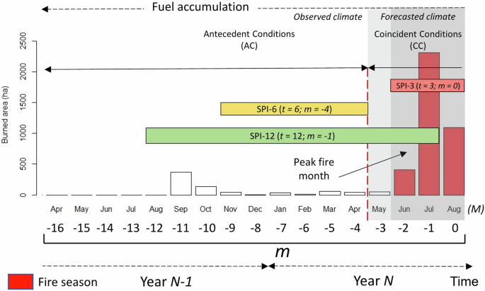
An example is shown for predicting the burned area (BA) anomaly during JJA (dark gray shading) for a specific grid point (longitude = 1°W, latitude = 41°N). The bars represent the average monthly burned area for the period 2001–2020 in Year N. This figure illustrates how climate observations and forecasts are combined to calculate the BA anomaly using the SPIt(M−m) as a predictor. The parameter t can take values of 3, 6, or 12 months, with the colors red, yellow, and green indicating SPI3, SPI6, and SPI12, respectively. This figure was generated using R software, version 4.3.1.
This modeling framework exploits different potential sources of fire predictability, delineating three key aspects. The first factor involves the relationship of burned area (BA) predictability with antecedent climatic conditions, those occurring before the BA season. As illustrated in Fig. 1, this concept is exemplified by the orange bar representing the 6-month aggregated Standardized Precipitation Index (SPI6) assessed in April. For instance, the BA anomalies for JJA (June–July–August) could be linked to the observed SPI6 values observed in April. The second dimension pertains to the influence of concurrent climatic conditions (visualized by the light gray shadow in Fig. 1), where the predictive accuracy of BA, as related to the SPI, improves with the extension of the accumulation period. This improvement is attributable to the incorporation of a broader period of observed data within longer SPI accumulations. Certain ecosystems may require an extended duration of dry conditions, including months preceding the fire season, to render the fuel sufficiently dry for fire propagation. In such scenarios, the forecast of drought conditions benefits from the incorporation of observed initial conditions with forecasted data. Figure 1 shows an example of issuing a BA anomaly forecast for JJA (denoted by the dark gray shadow). Here, BA predictability is linked to the SPI12, computed in August (green bar in Fig. 1), which includes observations from September through April combined with forecasts from May through August. In this case, the main sources of predictability come from the inherent persistence of drought and, therefore, its cumulative nature39,40,41. The last and least favorable conditions for skillful BA forecasting (i.e., when the area under the receiver operating characteristic curve, AUC, exceeds 0.5, with 1 being optimal; statistical significance is assessed using the Mann–Whitney U test with a p-value threshold of <0.01; see the “Methods” section) occurs when BA is associated with the SPI of the same season, as observed over the June–August period (SPI3; red bar in Fig. 1). In these instances, BA predictability relies solely on the SEAS5 seasonal forecasts, thus from the inherent capabilities of dynamical models for SPI forecasts, which exhibit a certain degree of accuracy for the initial month of predictions—stemming from inherent weather predictability—and generally show limited skill in subsequent months, typically restricted to tropical areas8,42, as detailed in Supplementary Fig. 1.
Forecast verification results
From an operational perspective, it is essential to assess whether the model can differentiate between positive and negative anomalies. For this, we use the Area Under the ROC Curve (receiver operating characteristic, AUC)43,44, a method widely used in fire prediction studies (see, e.g., refs. 11,45). The ROC curve compares the hit rate (when a forecasted event occurs) with the false alarm rate (when an event is forecasted but does not occur).
Figure 2a, b shows that the climate-burned area model exhibits significant predictive skill in DJF and JJA, hovering between 66% and 70% of the evaluated domain, respectively (see Supplementary Fig. 2a, b for the MAM and SON results, with 68%). The median AUC, calculated at statistically significant grid points, is around 0.88 (with 1 being the optimal value). These results reflect the maximum skill of the prediction system, derived from an out-of-sample analysis using cross-calibration and validation. That is, this is the skill level if we feed the model with “perfect” seasonal forecasts (observations, as done in this case).
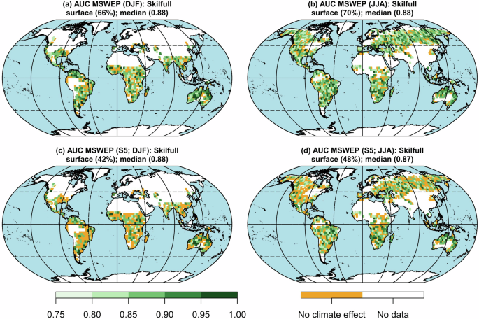
Panels a and b correspond to the periods December–January–February (DJF) and June–July–August (JJA), respectively, when the model is fed with observations. Panels c and d show the same periods, but the model is fed with seasonal forecasts. The grid points in orange indicate non-significant AUC values (p-value ≥ 0.01). The white color considers those grid points where the seasonal burned area equals zero in less than half of the available period (i.e., BA = 0 in <10 out of 20 years). This figure was generated using R software, version 4.3.1.
On the other hand, Fig. 2c, d shows the system’s performance when fed with seasonal forecasts. Although there is a reduction in the percentage of the domain with statistically significant values, the system still demonstrates predictive skill in a considerable portion of the domain (42% for DJF and 48% for JJA; see Supplementary Fig. 2c, d for the MAM and SON results, with 48% and 49%, respectively). The median AUC remains around 0.87/0.88 across all seasons. The skill map of the predictions is noisier compared to the observations, which is due to the overlap of two data layers: one where there is a link between BA and SPI (based on observations) and another where seasonal forecasts show skillful results (shown only in areas with a significant AUC). This overlap can result in alternating patterns of significant and non-significant cells, especially in certain regions or seasons (such as Africa in DJF or North America in JJA) while in others, such as Australia in SON or South America in JJA, greater spatial coherence is observed.
Figure 3 provides a detailed analysis of the model’s performance in specific regions (following ref. 46 see Supplementary Fig. 3). Figure 3a–d present DJF, MAM, JJA, and SON seasons, with box plots showing the spatial distribution of observations (in light pink) and predictions (in orange). Overall, the AUC values for the model with observations are high and consistent across all seasons. The medians exceed 0.8 in all regions. Australia and New Zealand (AUST) and Northern Hemisphere South America (NHSA) stand out in DJF and JJA, with values close to 0.9 (Fig. 3a, c). In SON, Equatorial Asia (EQAS) reaches values as high as 0.95 (Fig. 3d). Regarding the bars representing the percentage of the area where the model with observations shows skill, all regions exceed the 55% threshold. AUST and NHSA stand out in DJF, explaining 84% of the area. In MAM (Fig. 3b), NHSA and Boreal Asia (BOAS) cover 76%. During JJA, AUST, and EQAS exceed 79%, and SON, AUST, and BOAS explain more than 75%. The poorest performances are observed in the Middle East (MIDE) and Central Asia (CEAS), where the areas explained do not exceed 65%. In DJF, CEAS barely reaches 55%, while MIDE shows a similar performance in SON. When the model incorporates seasonal predictions, although the AUC values remain high, the percentage of the area explained decreases across all seasons and regions. The largest reductions are seen in EQAS, dropping from 71% to 29% in DJF, and in NHSA, which falls from 84% to 49% in MAM. Despite this, AUST maintains good performance. In JJA and SON, it continues to explain 71% of the area. The poorest results in terms of the area explained are observed in Europe (EURO), covering only 32% and 33% in SON and DJF, respectively.
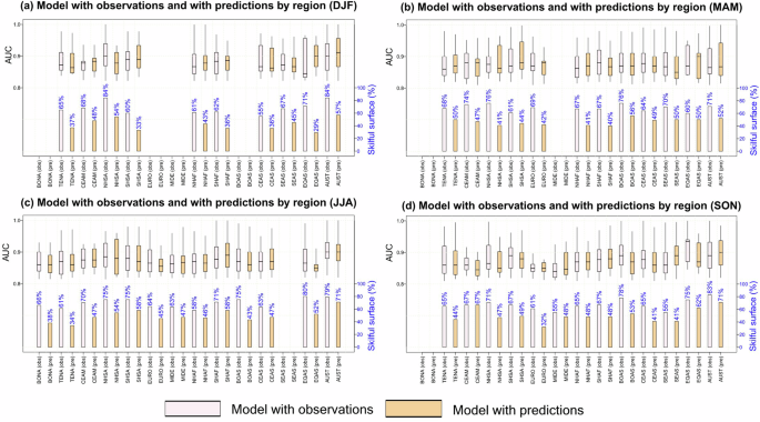
Panels a–d show the distribution of AUC (area under the ROC curve) values for the model based on observations (obs, in white) and predictions (pred, in orange) across different seasons: Panel a December–January–February (DJF), panel b March–April–May (MAM), panel c June–July–August (JJA), and panel d September–October–November (SON). The median is shown as a solid line, the squares indicate the interquartile range (25–75th percentile), and the ends of the whiskers represent the 5–95th percentile range. The percentages in blue indicate the proportion of the surface area with significant predictive skill (p-value < 0.01) in each region (Supplementary Fig. 3). The bars at the bottom of the graphs show the percentage of the significant domain. This figure was generated using R software, version 4.3.1.
To assess the effectiveness of the random forest (RF) model, Fig. 4 compares its performance with a logistic regression (LR) model. Figure 4a shows the performance of the models based on observations. AUC values are consistently high in all seasons for both methods (RF and LR). In particular, RF shows slightly higher AUC values compared to LR. Also, the bars indicate that the significant area is considerably higher for RF in all seasons, reaching a maximum of 70% in JJA. On the other hand, LR shows lower significant areas compared to RF, with a maximum of 48% in SON. Figure 4b shows the performance of the models with seasonal predictions. Like the models with observations, AUC values are high for both methods in all seasons. However, there is a reduction in AUC values and in the significant area compared to the models with observations. RF again shows superior performance, with significant areas reaching up to 49% in SON, while LR shows a lower percentage of significant areas with a maximum of 31% in SON. A common feature is that the skill is similar among the target seasons. For a more detailed spatial analysis of LR, see Supplementary Fig. 4 for the model with observations and Supplementary Fig. 5 for the model including seasonal predictions. Supplementary Table 1 compares the AUC performance between RF and LR models, categorized by season and region, for both observation-based models (Supplementary Tables 1a–d) and prediction-based models (Supplementary Tables 1e–h). In all cases, RF outperforms LR, although the differences vary by region and season. For example, when the model is based solely on observations, RF is more effective in Central Asia (CEAS) and Equatorial Asia (EQAS), dominating more than 96% of the domain’s surface in DJF and MAM, respectively. When including predictions, RF maintains its advantage, covering 100% of the domain’s surface in EQAS during DJF and 87% in Northern Hemisphere South America (NHSA) during JJA. On the other hand, LR narrows these differences in certain regions, such as Northern Hemisphere Africa (NHAF) during JJA, where it covers 46% of the domain’s surface with observations, and EQAS during SON with predictions, where it covers 41%. This superior performance of RF is due to its ability to capture complex nonlinear relationships and its robustness in combining multiple models (500 trees), which enhances generalization and reduces variance.
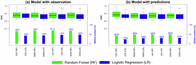
Panel a shows the models with observations and panel b shows the models with seasonal predictions. RF is represented in green and LR is represented in blue. The boxplots show the spatial distribution of significant AUC values. The median is shown as a solid line, the squares indicate the percentile range 25th–75th, while the whiskers show the percentile range 5th–95th. The bars at the bottom of the plots indicate the percentage of the significant domain (p-value < 0.01). This figure was generated using R software, version 4.3.1.
Climate-burned area model characteristics
The obtained results are influenced by the accuracy of climate observations22,23, burned area observations47,48,49, SPI estimation37, as well as the characteristics of the climate-burned area model8, which play a crucial role in how these variables interact. In this context, Fig. 5 presents the Spearman correlation coefficient between BA and the best SPI (i.e., the SPI aggregated over the period that maximizes the model skill, see the “Methods” section). Negative correlation values are associated with drought conditions (as drought conditions are indicated by negative SPI values), suggesting that drought conditions increase the anomaly of the burned area. Positive correlation values are associated with wet conditions, indicating that they can also influence the burned area, possibly due to increased vegetation38,50,51,52. That is, there are regions where fire spread is mostly limited by the fuel amount, which may be enhanced by antecedent wet conditions. The results show that ~53% of the domain presents a negative correlation (depending on the season; see Supplementary Fig. 6a). During DJF (Fig. 5a) positive correlations are prominent in Western Australia and Patagonia, coinciding with arid areas. In MAM (Fig. 5b), the domain extends to the extratropical regions of the Northern Hemisphere, expanding the relationship between drought and fire anomalies to North America and Eurasia (i.e. negative correlations). In JJA (Fig. 5c), the intensity of the negative correlation increases in the extratropical regions of Asia, coinciding with the boreal summer, while the southwestern region of Asia shows positive correlations. In the tropical regions of the Southern Hemisphere, positive correlations intensify in Australia and near the Kalahari Desert. Finally, in SON (Fig. 5d), the influence of drought is accentuated again in the Southern Hemisphere, especially in Indonesia and South America, coinciding with the beginning of the austral spring.
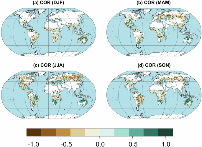
Panels a–d correspond to DJF, MAM, JJA, and SON, respectively. Grid points are shaded in gray when the model is not significant (p-value ≥ 0.01), while white is used for those points where the seasonal BA is equal to zero in less than half of the analyzed period (i.e., BA = 0 in < 10 of the 20 years). This figure was generated using R software, version 4.3.1.
Supplementary Fig. 6b shows the values of m, which represent the most influential month on the burned area anomaly, either before the fire season (AC, m = −16 to −4) or during the season (CC, m = −3 to 0). In all seasons, more than 63% of the influential months occur before the fire season, due to the greater number of preceding months (13) compared to concurrent months (4). However, CC months have a greater individual impact, suggesting they are more relevant in the short term for fire anomalies. Supplementary Fig. 7 illustrates this behavior by region: in DJF, concurrent months influence most regions, while AC months dominate only in Center America (CEAM). In JJA, CC months mainly affect regions in the Northern Hemisphere (boreal summer), whereas AC months have more influence in the Southern Hemisphere (austral winter). Supplementary Fig. 6c presents the drought index used, the SPI (3, 6, or 12 months), which indicates whether fires respond to short-, medium-, or long-term droughts. In general, SPI3 (short-term) is the most influential, especially in DJF, MAM, and SON, covering ~40% of the area. Only in JJA does SPI6 (medium-term) exceed SPI3 in relevance, at 36%. Supplementary Fig. 8 details the SPI variation by region: in DJF, SPI3 dominates tropical areas such as Northern Hemisphere South America (NHSA) and Australia and New Zealand (AUST; 50–60%), while SPI12 is significant in Temperate North America (TENA) and Southern Hemisphere South America (SHSA; ~40%). In MAM, JJA, and SON, SPI12 is key in AUST, exceeding 40%, while SPI3 and SPI6 are more relevant in extratropical regions such as Boreal Asia (BOAS) and Europe (EURO; ~40%). SPI3 generally remains the most important in tropical regions throughout the year.
The increase in t values significantly improves the predictive ability of the SPI. This is because the prediction utilizes more observed data for longer SPI accumulation windows. This approach combines observational data from the months preceding the fire season with seasonal forecasts specific to the fire season (see Supplementary Fig. 1). Such a method is particularly valuable in regions where dynamic forecasting systems still present significant errors, such as in mid-latitude areas (see, e.g., refs. 42,53,54). In summary, the results of this study align with those of ref. 52, indicating that the relationship between climatic conditions and burned area anomalies varies considerably by season and region. This variability reflects the effectiveness of using SPI across different timescales, as highlighted by the influences of m and t. In humid areas, concurrent droughts during the fire season increase the burned area, while in arid regions, such as Australia and parts of South America, antecedent wet conditions are key to increasing fuel availability and, consequently, the extent of the burned area. In this context, the predominance of SPI3 in tropical regions and SPI12 in extratropical and arid areas underscores the importance of drought timescales for predicting fire activity. In humid zones, short-term droughts dominate fire behavior, whereas, in drier areas, antecedent wet conditions heighten the likelihood of larger fires. These findings highlight the crucial role of both antecedent and concurrent droughts in better understanding burned area anomalies and optimizing prediction models across varying climatic contexts.
Figure 6 provides an example as a case study. It focuses on the analysis of the JJA season for the year 2012, selected for presenting the highest positive fire anomaly during the period of study (2001–2020), affecting around 57% of the studied domain. The anomaly in burned area in 2012 could be linked to extensive long-duration droughts (SPI12) that affected regions such as Temperate North America (TENA), Boreal Asia (BOAS), Southern Hemisphere South America (SHSA), and Southern Hemisphere Africa (SHAF), as well as short-duration drought conditions (SPI3) in Australia and New Zealand (AUST; see ref. 23; https://www.um.es/gmar/projects/predfire-viewer.html). These regions generally coincide with the areas where a positive burned area anomaly was observed, as shown in Fig. 6. This set of maps illustrates various aspects of the BA anomalies and the model’s response to these extreme conditions. Specifically, Fig. 6a displays the burned area anomaly; Fig. 6b reflects the probability, according to the model, of a BA anomaly occurring; Fig. 6c illustrates the alert level of the model, determined using the methodology employed by ref. 45. The threshold is defined as the probability level that maximizes the difference between the rate of detection of actual fires and the rate of false alarms. Consequently, all probabilities that exceed this threshold are considered alerts. Figure 6d shows the results through verification of the alert by means of the contingency table that quantifies the true positives (48%; Light green color), false positives (16%; yellow color), false negatives (15%; orange color), and true negatives (21%; dark green color).
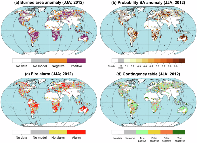
Panel a Burned area anomaly; panel b Probability of a burned area anomaly occurring according to the model with S5; panel c Alert level of the burned area anomaly; panel d Alert verification through a contingency table. The gray color represents where the model fed with predictions is not significant (p-value ≥ 0.01). The white color considers those points of the grid where the seasonal BA is equal to zero in less than half of the available period (i.e. BA = 0 in <10 of the 20 years). This figure was generated using R software, version 4.3.1.
Finally, for a detailed breakdown of these results by region, refer to Supplementary Table 2. The Northern Hemisphere South America (NHSA) and Central America (CEAM) regions show the highest errors, with 54% and 50% of the surface, respectively, mainly due to false positives. In NHSA, 46% of the surface corresponds to false positives, indicating an overestimation of fires, while CEAM has 36% of its surface with false positives. Regarding the model’s success, Australia and New Zealand (AUST) stands out with 85% of the surface correctly predicted, followed by Boreal North America (BONA) and Southern Hemisphere South America (SHAF) with rates of 70% and 69% of the surface. Although SHAF performs well, it has 29% of its surface with false negatives, indicating some difficulties with the model.
Discussion
This study introduces an innovative approach for the seasonal prediction of burned area anomalies using random forest (RF). The system combines the standardized precipitation index (SPI)37 with seasonal dynamic predictions (SEAS5)36 to anticipate drought weather conditions, which act as a predictor of burned area anomalies. This process is optimized for producing seasonal predictions with a 4-month horizon, allowing forecasts to be issued one month before the start of the target seasons. The developed model shows significant predictive capability across much of the evaluated domain, covering 68% of the burned area using only observational climate data. This capability highlights the decisive influence of weather patterns on the dynamics of forest fires8,38,52.
We consider SPI to be suitable for our analysis, as it has proven to be as effective as the standardized precipitation evapotranspiration index (SPEI)55,56 globally and has shown better performance than temperature in this type of prediction (see ref. 8), providing a simpler model. Also, the feedback between precipitation and temperature/evaporative demand supports the use of only SPI (see e.g., ref. 57). In addition, for practical applications, such as integrating fire danger prediction into operational systems, SPI offers a simpler and more accessible metric facilitating its applicability across diverse climatic regions. However, more complex options could be explored in future work, such as those proposed by ref. 52 who suggest identifying the most suitable variable depending on the study region.
Due to limitations in the skill of seasonal fire prediction models, we adopt the less demanding approach of modeling anomalies rather than absolute burned area, as done in previous studies on seasonal fire forecasts (e.g., refs. 11,58). Furthermore, satellite-derived burned area datasets, including those used in this study, face significant challenges in detecting small fires and accurately quantifying the total burned area, particularly in hotspot regions such as Africa (e.g., refs. 59,60). By focusing on anomalies at a relatively coarse resolution (2.5° × 2.5° grid) instead of absolute burned area values, this approach helps mitigate the influence of systematic errors. Nevertheless, developing a model capable of predicting positive and negative anomalies months in advance and on a global scale is often sufficient for triggering alerts and prioritizing interventions. This approach provides actionable insights for early warning systems and resource planning. For instance, ref. 5 demonstrated the practical utility of an anomaly-based seasonal prediction system for summer wildfires in a Mediterranean region, successfully integrating a participatory approach with end-users. This highlights how anomaly-based systems effectively balance simplicity and operational relevance. Future studies could explore modeling absolute burned area, particularly as more precise satellite datasets and high-resolution regional data become available.
The system’s skill is evident in regions such as Australia or northern South America, where the observation-based model can predict up to 84% of the domain, depending on the season. In Africa, the model covers up to 71% of the domain, which is significant given that this continent has the largest burned area globally, contributing significantly to carbon emissions from wildfires60,61,62,63. The use of the MSWEP dataset26, which integrates rainfall station data, satellite estimates, and reanalyses, has helped reduce uncertainty in drought observations, particularly on this continent20,23,26,42,64,65.
On the other hand, when fed with seasonal forecasts like SEAS5, the model’s predictive skill depends on the SPI time scale, being lower for short-term forecasts, particularly within the same season. Although predictability significantly decreases beyond the first month, SEAS5 performs better than empirical methods, which rely on statistical relationships derived from historical records41,66. While these methods have shown utility as a reference and demonstrated skill in previous studies (e.g., refs. 24,42,54) they face important limitations. They assume stationary climatic conditions and depend heavily on the quality and availability of historical data, which reduces their applicability in regions with limited data or under changing climate scenarios25,42,67. In contrast, SEAS5 incorporates dynamic initial conditions and physical processes, providing greater adaptability to non-linear climatic variations and better capturing conditions in regions influenced by teleconnections such as ENSO36,68. This approach is particularly useful in subtropical regions such as Australia and South America42, where the model more accurately captures complex climatic patterns36,66. In Africa, although the percentage of AUC-significant areas is lower compared to other regions (around 40%, depending on the season), the model’s performance remains relevant.
Our approach, using RF, not only improves prediction accuracy but also optimizes the use of observational data and seasonal predictions without incurring substantial computational costs. Additionally, RF significantly outperforms the predictions achieved by the logistic regression (LR) model. In summary, this study demonstrates the effectiveness of RF in improving seasonal fire prediction. This advanced approach holds great potential for practical applications in global fire management and prevention, offering a valuable tool for decision-making based on more accurate and reliable predictions.
Methods
Precipitation data
For this study, the multi-source weighted-ensemble precipitation database (MSWEP v.2.826) was used. This dataset is derived from the amalgamation of rain gauge measurements, satellite estimates, and numerical reanalyzes. We chose MSWEP as recent studies have confirmed its superior performance in comparison to other global precipitation datasets23,27,69. Meteorological drought was assessed using the standardized precipitation index (SPI)37. The SPI calculation was performed using the R SPEI package70, fitting precipitation data to a gamma distribution as recommended by the World Meteorological Organization71.
SEAS5 prediction system consists of 25 ensemble members from 1993 until December 2016, referred to as re-forecasts. After that period, they consist of seasonal forecasts with 51 members. It is important to note that the re-forecast dataset was initialized using ERA-Interim analysis data, while forecast simulations from 2016 onward are initialized using ECMWF operational analysis. Therefore, there is an inconsistency between 1993–2016 and the 2017–2020 period. For both the re-forecast period (1993–2016) and the forecast period (2017–2022), the temporal resolution is daily forecasts, available once a month, with a prediction horizon of 216 days (equivalent to 7 months). However, there is a difference in the number of ensemble simulations, with the re-forecast providing only 25 ensemble members compared to the 51 of the forecast period. To ensure equivalence between the periods, only the first 25 ensemble members of the forecast have been retained72.
Following the methodology proposed by ref. 8 MSWEP estimates were integrated with the dynamic forecasts through the following steps: (i) precipitation values were reassigned from their original resolution to a 2.5° × 2.5° grid using first-order conservative remapping73; (ii) forecast data bias was adjusted using a leave-one-year-out linear scaling, based on the comparison between the long-term averages of the observed and simulated data; (iii) accumulated precipitation values for periods of 3, 6, and 12 months were calculated by integrating the observed and remapped data (excluding those from the trial year); and (iv) the SPI was calculated for these periods. For example, to predict the SPI6 in May (a prediction with a 4-month lead time), the observed precipitation in March and April was summed with the forecasted values for May, June, July, and August (see Fig. 1). This procedure was repeated for the 25 members of the SEAS5 ensemble, resulting in 25 distinct SPI estimates. The estimation of the SPI for both MSWEP observations and forecasts was carried out from 1993 to 2020.
Burned area data
Monthly burned area data are obtained from the FireCCI database version 5.1 (FireCCI51)74. FireCCI51 has a spatial resolution of 0.25° and covers the period 2001–2020. We applied this pre-processing to the BA data: (i) the BA on cropland is excluded due to its complexity in being mapped accurately using satellite data and because cropland fires tend to be small, display less interannual variability, and generally are influenced by variations in crop selection, policy decisions, and agricultural methodologies38; (ii) BA data are remapped summing all grid points to a resolution of 0.25° within a grid point of 2.5°; (iii) BA data are aggregated into seasons (December–January–February, DJF; March–April–May, MAM; June–July–August, JJA; September–October–November, SON), considering grid points where seasonal burned area is different from zero in half or more of the available period (i.e., burned area > 0 in at least 10 out of 20 years), following the ref. 6,8.
Defining the climate-burned area model
We develop individual models for each 2.5° × 2.5° grid cell as detailed below. We applied the machine learning algorithm ‘Random Forests’ (RF)28 to time series of fires and climate predictors to predict anomalies in the burned area. The target variable is BA anomaly, being defined as BA below- or above the 50th percentile. This non-parametric statistical method utilizes a collection of decision trees and is suitable for both regression and classification28. RF works by constructing multiple decision trees during training and using majority voting (for classification) or averaging (for regression) of the individual tree predictions to obtain the final prediction. In our analysis, we utilized the “randomForest” package version 4.7-1.1 in R to implement the RF algorithm. The RF parameters were configured with their default values to balance model complexity and computational efficiency. Specifically, the parameter mtry (i.e., the number of predictor variables randomly selected) was set to 1, given that we have only one predictor in our model. This setting ensures that each decision tree in the forest considers one randomly selected feature at each split. We set the ntree parameter (i.e., the number of trees averaged in the ensemble forest) to 500, indicating that 500 decision trees were constructed for each RF. This number of trees was chosen to ensure the stability and accuracy of the model’s predictions. A larger number of trees generally improves the model’s performance by reducing variance, though it also increases computational cost. In our context, 500 trees provided a robust model without excessive computational demand. Additionally, parameters such as nodesize and maxnodes were kept at their default settings. Specifically, nodesize is set to 1 for classification, ensuring that each terminal node contains at least one observation. The maxnodes parameter is not explicitly set, allowing the trees to grow fully. In this case, the maximum number of terminal nodes is ~2 × n−1, where n is the number of observations in the training dataset28.
To identify the most effective model, we evaluated all possible combinations of predictors SPIt(M-m) where t corresponds to the cumulative time of SPIt (t = 3, 6, 12) and M−m is the month for which SPI is calculated. We considered that (i) M is the last month of the analysis season (i.e., 2 for DJF, 5 for MAM, 8 for JJA, and 11 for SON) and (ii) m = −16, −15, …, −1, 0; where 0 corresponds to the last month of the analysis season (in line with previous studies, see, e.g., refs. 8,38,52).
We explored all possible aggregations of the predictors through an out-of-sample calibration. This involves excluding one year from the study period (2001–2020) and training the model with data from the remaining years (n−1 years). The excluded year is used as a validation set, and this process is repeated iteratively for each year in the study period. In each iteration, the Random Forest model is trained with the training data and evaluated using predictions on the validation set. Finally, the dynamic seasonal predictions are incorporated only at those grid points where the best m corresponds to the fire season (m < −3). Since the model is calculated for the 25 SPI predictions of the SEAS5 system, 25 probabilities of burned area anomaly are obtained. To evaluate the model’s performance, the mean of these 25 probabilities is used.
The performance of the model is evaluated using the area under the receiver operating characteristic curve (AUC)43,44, similar to other fire prediction studies (e.g., refs. 5,11). This metric indicates whether the model outperforms randomness, with 1 being the optimal value. The significance of the AUC is determined using the Mann–Whitney U test44, considering a p-value < 0.01 as significant. Additionally, we employed Spearman’s correlation to analyze the relationship between the best SPI identified by RF and the burned area. For a better interpretation of the results, the model evaluation is presented by regions, using 14 regions defined by ref. 46. To ensure a robust analysis, it has been established that at least 10% of the surface area of each region must exhibit anomalies in burned areas during the season. That is, regions with limited data have not been included in the analysis, as a low number of observations could lead to unrepresentative or distorted results, limiting the ability to draw reliable conclusions about the model’s performance.
Finally, we verified the robustness of our results by comparing the RF model with a logistic regression model (LR), as described in Supplementary Material. The latter links climate variables with BA anomalies, defining BA as below or above the 50th percentile. This is a common approach in fire modeling (see, e.g., refs. 5,8,11,58,75) to link climate and fire anomalies (Eq. 1):
where p represents the probability that the BA is above the median. The intercept of the model is β0, while β reflects the sensitivity of BA to SPI; the term ε represents a stochastic noise component that accounts for other processes affecting BA, beyond SPI. A critical step in the development of these empirical models is to find whether the BA anomaly depends on SPI and what are the best time windows to estimate SPI. To resolve this, we consider different temporal aggregations of the predictors by cross-calibration in leave-one-year-out mode8,76.
Responses