Equatorial convection controls boreal summer intraseasonal oscillations in the present and future climates

Introduction
Indian summer monsoon rainfall (ISMR) is responsible for most of the country’s agricultural yield1. The monsoon period (June-July-August-September, JJAS) is characterized by intense convection, leading to widespread precipitation throughout the country. This precipitation is not continuous in time and is characterized by a series of wet and dry periods called active and break spells, respectively2,3,4,5,6. While the extended dry period leads to drought, the extended wet period leads to flood7. These dry and wet periods are modulated by the Boreal summer Intraseasonal Oscillation (BSISO), which is the dominant mode of intraseasonal variability in the Indian summer monsoon8,9,10. While a relationship between BSISO and wet/dry spells exists for most of the regions of the country, it is more pronounced over the core monsoon zone.
The BSISO’s wet spell is initiated in the equatorial Indian Ocean and moves northward over to the Indian land mass and adjoining ocean basins, bringing rainfall11,12. Many possible mechanisms for the northward propagation have been put forward in the past13,14,15,16,17,18,19. The northward propagation of BSISO is considered the unstable mode of monsoon flow, and this instability is mainly controlled by the background zonal wind shear17,19,20,21. The background easterly zonal wind shear generates barotropic vorticity to the north of the convection centre, and this vorticity then induces a boundary layer convergence, moving the convection northward17,22. An eigenvalue analysis shows that the BSISO always propagates northward in the presence of easterly wind shear17.
However, it has been suggested recently that even with a conducive background shear, a weak BSISO convective signal at the equator dissipates without significant northward propagation23,24. A few studies also suggested the organization of BSISO convection22,25 is important for the northward propagation of BSISO in the CMIP6 models. Thus, this study aims to establish the role of equatorial convection in the northward propagation of BSISO.
Nevertheless, establishing this is not straightforward, given that not all the models of CMIP6 faithfully reproduce the BSISO’s northward propagation22,25,26,27. From the inception, CMIP models had difficulty in faithfully capturing the BSISO, with only 2 of the 17 evaluated models showing some appreciable skill in BSISO’s simulation in CMIP2+ and CMIP328. While observations suggest that, often, northward propagation of BSISO is associated with eastward propagation into the West Pacific29, the CMIP3 models produced northward propagations without eastward propagation30. The situation improved with the CMIP5, with more models simulating the northward propagation of BSISO. However, many models underestimate the BSISO variance in the equatorial Indian Ocean31. This underestimation of BSISO variance is still found in CMIP6 models, with only 10 out of 19 evaluated models capturing the northward propagation22. However, this inherent inability of some models allows us to pursue further the hypothesis that equatorial BSISO convection also has an essential role in the northward propagation of BSISO.
Finally, after establishing the role of equatorial convection in northward propagation, we also answer the question, “What would be the future of BSISO in the Indian Ocean basin?”. Understanding the future of BSISO is essential as it has been established recently that the large-scale BSISO environment enormously enhances the probability of extreme rainfall events32. The enhancement of rainfall caused by low-pressure systems (LPS) during certain phases of BSISO has been reported33. Thus, answering the above question helps better predict extreme rainfall events and mitigate their impact.
Recently, it has been argued that BSISO and Madden-Julian Oscillation (MJO) manifest the same low-frequency variability in different background moisture states34,35,36, and capturing moisture dynamics is crucial for MJO prediction37. Hence, in this work, we examine the moisture dynamics in the CMIP6 models. Using a counting algorithm to determine the number of northward propagations in each of the selected CMIP6 models, we categorize the models into above-average-performing models (AAPM) and below-average-performing models (BAPM) based on the percentage of northward propagations from the equator in each model (Section “Data and Methods”). We perform a composite moisture budget to understand the difference in northward propagations in AAPM and BAPM composites. Finally, we use the SSP370 projections from the available AAPMs to illuminate the future of BSISO. We chose the SSP370 because we are a little optimistic about the climate action being taken worldwide; since extreme events are on the rise worldwide, we expect countries worldwide to act, thereby cutting off carbon emissions. Additionally, SSP370 is a newly added scenario in the CMIP6 that was added to bridge the gap between RCP6.0 and RCP8.5 in the CMIP5 and was studied relatively less compared to SSP585.
Results
Difference in propagation characteristics between AAPM and BAPM composites
Using a simple counting algorithm (Section “Data and Methods”), we identify 12 models as AAPMs and the remaining 8 as BAPMs. Figure 1 shows the composite of propagation for the AAPMs and the BAPMs. Despite a similar evolution trend between the AAPM and BAPM composites, the AAPM composite exhibits a strong equatorial rainfall structure on day 0. Both composites capture the weakening of rainfall anomalies across the South Bay of Bengal (SBoB)38. However, the rainfall anomaly strengthens considerably at further lead times over the North Bay of Bengal in the AAPM composite compared to the BAPM composite (day 12), which gives confidence in the algorithm we used for categorisation. We find that 56% of events at the equator propagate northward in the AAPM composite, whereas this proportion is only 35% for the BAPM composite. While the number of northward propagations in the observations stands at 62% (Table 2).

Evolution composites of the ISO-filtered rainfall anomaly (mm/day, shading) and the ISO-filtered wind anomaly (m/s, vectors) for (a) AAPM and (b) BBPM. Shading is only done if the values are significant at 95% using a two-tailed t-test. Wind vectors are plotted for all the values irrespective of significance. Day 0 corresponds to the day of maximum convection as described in Section “Data and Methods”. The days relative to day 0 are printed in the bottom right of each plot, and reference vectors are printed on the right top of each panel.
Moisture budget
A positive moisture tendency develops to the north of the convection centre, which moistens the atmosphere to the north of the convection centre, helping prime the atmosphere for deep convection and thus assisting northward propagation23,35,39. Therefore, we conduct a vertically integrated moisture budget to understand the difference between the propagations in AAPM and BAPM composites. Figure 2 shows the result from the moisture budget. The budget is evaluated on day 0, corresponding to the day of maximum ISO rainfall across the equator. It becomes apparent that the moisture tendency to the north of the rainfall centre is stronger in the AAPM composite than in BBPM. Also, the tendency is collocated with the horizontal moisture advection (Fig. 2a, b). In contrast, the precipitation roughly balances the vertical advection of the moisture (Fig. 2c). However, evaporation is opposite in phase to the tendency and horizontal advection (Fig. 2d). In conclusion, the moisture tendency is maintained by horizontal advection, and the reduced tendency in the BAPM composite causes weaker propagations in the composite.
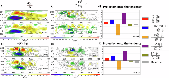
Panels a–d represent tendency, horizontal advection, columnar processes (Eq. (2)), and evaporation, respectively. Stippling in panels a–d represent values significant at 95% using a two-tailed t-test. Contours in panels b–d show the moisture tendency overlaid on each term. Solid contours represent positive tendency, and the dashed contours negative tendency. The projection of each budget term onto the tendency term is shown in e for AAPM and f in BAPM. Refer to Supplementary Fig. 13 for the scaled version of the figure.
To confirm the above findings, we project each term in the budget onto the tendency (Eq. (7), Fig. 2e, f). The relative contribution of the horizontal advection to the tendency remains the same, with the precipitation and vertical advection balancing each other in both cases, which can be seen much more clearly when we project all the terms onto the precipitation (Supplementary Fig. 2). This means that the change in the relative contribution from the other terms does not cause the observed reduction in the tendency. Instead, the weaker tendency in the BBPM composite is due to reduced horizontal advection.
Contribution to horizontal advection
Further, we break down the horizontal advection into zonal and meridional advection (Eq. (4), Fig. 3). In both AAPM and BAPM composites, zonal advection positively contributes to the moistening to the north of the convection centre with a predominant signature in the Arabian Sea (Fig. 3a). In contrast, the meridional advection predominantly moistens the Bay of Bengal (Fig. 3e). Both zonal and meridional advection show a considerable reduction in BAPM models.
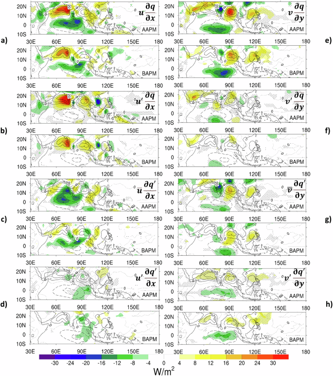
Breakdown of zonal (a–d) and meridional advection (e–h) into the respective components (Eqs. (5) and (6)) for AAPM and BAPM. Stippling represents values significant at 95% using a two-tailed t-test. Contours show the horizontal advection term (L.H.S of Eq. (4)) from −30 to 30 W/m2 in steps of 10. solid contours show a positive tendency and dashed contours show a negative horizontal advection. Refer to Supplementary Fig. 14 for scaled version of the figure.
To further understand the processes responsible for the reduction of the advection in the BAPM composite, we split the zonal and meridional advection into respective components (Eqs. (5) and (6), Fig. 3). The significant contribution to the zonal advection comes from the advection of background moisture by zonal wind perturbation (left({u}^{{prime} }frac{partial overline{q}}{partial x}right)). At the same time, the remaining two terms do not contribute much to the moistening. The weaker ({u}^{{prime} }frac{partial overline{q}}{partial x}) term results in weaker zonal advection in the BAPM composite.
Most of the contribution to meridional advection comes from the advection of anomalous moisture by the background meridional wind (left(overline{v}frac{partial {q}^{{prime} }}{partial y}right)). Unlike the zonal advection, the other two terms of the meridional advection also contribute to moistening ahead of the convection centre. Figure 3f, g, shows that (overline{v}frac{partial {q}^{{prime} }}{partial y}) and ({v}^{{prime} }frac{partial overline{q}}{partial y}) are weaker over the Bay in the BAPM composite. We also compare the spatial pattern of various terms with the ERA5 reanalysis (Supplementary Fig. 4). Interestingly, the spatial pattern of all the terms remains similar to the AAPM composite, albeit with a larger magnitude, which explains why a larger proportion (62%) of the events propagate northward in observations (Table 2).
To understand the weaker ({u}^{{prime} }frac{partial overline{q}}{partial x}) and ({v}^{{prime} }frac{partial overline{q}}{partial y}) terms in the BAPM composite we construct the vertically integrated background specific humidity and day 0 wind perturbations at the 850 hPa level (Fig. 4). The background moisture is not significantly different between AAPM and BAPM composite (Fig. 4a, b), except for slightly larger moisture over North India (Fig. 4g). The meridional (Fig. 4d–f) and zonal gradients (Fig. 4h–j) look similar between AAPM and BAPM composites. Thus, the reduction in the above two terms stems from the decrease in the wind perturbations, as seen from the vectors in Fig. 4c. The stronger wind perturbations in AAPM cause a stronger advection of background moisture. Next assessing the (overline{v}frac{partial {q}^{{prime} }}{partial y}) term, we note that the gradient (left(frac{partial {q}^{{prime} }}{partial y}right)) is more significant in the AAPM composite along with the stronger background meridional wind at the 700 hPa level than the BAPM composite (Fig. 4g, k), leading to stronger moisture advection.
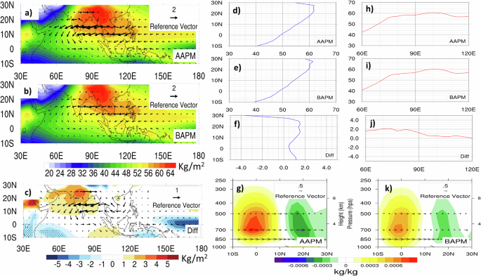
Background (JJAS mean) vertically integrated moisture (shading, kg/m2) of AAPM (a) BAPM (b) and the difference between the two (c). The stippling in (c) shows the values significant at 95% using a two-tailed Student’s t test. Meridional structure of the vertically integrated moisture in AAPM (d) BAPM (e) and the difference between the two (f) averaged over the longitudes 80°E − 95°E; the Y-axis represents the latitude. The zonal structure of the vertically integrated moisture for AAPM (h) BAPM (i) and the difference between the two (j) averaged over the latitudes 10°N − 20°N; the X-axis represents the longitude. g and k represent the day 0 vertical structure of ISO-filtered specific humidity anomalies (kg/kg) and JJAS mean meridional winds for AAPM and BAPM, respectively.
Hence, the difference in the horizontal advection between AAPM and BAPM composites can be mainly attributed to the perturbations ({u}^{{prime} }), ({v}^{{prime} }) and (frac{partial {q}^{{prime} }}{partial y}). The ISO circulation anomalies resemble a modified Gill response, with stronger convective heating to the north of the equator, resulting in a stronger Rossby vortex lobe to the north of the equator40. This response is stronger in the AAPM composites because of stronger equatorial convection to the north of the equator in the AAPM composite (Supplementary Fig. 9). Thus, the wind perturbations (left({u}^{{prime} },{v}^{{prime} }right)) associated with the Rossby vortex are stronger in the AAPM composites. On the other hand, the (left(frac{partial {q}^{{prime} }}{partial y}right)) is more significant since the AAPM composite’s larger rainfall necessitates a larger moisture perturbation (Fig. 4g, k).
We also examine the same in the observations and ERA5 data. The Rossby vortex lobes and the associated wind perturbations in the observations are even stronger than the AAPM composite (Supplementary Fig. 3) because of stronger ISO convection in the observations. As already discussed, this leads to stronger advection and a larger proportion of northward propagations in the observations. Thus, in conclusion, the difference in the propagation characteristics between AAPM and BAPM composites is mainly controlled by the strength of the equatorial convection in respective models.
Future of the BSISO
Next, we try to answer the question, “What changes would we likely be seeing in the structure and intensity of the BSISO?” in the warming climate scenario. We use SSP370 projections to answer the question. SSP370 scenario corresponds to a 7 W/m2 anthropogenic warming by the year 2100 and implies high challenges to mitigation and adaptation41. Only 6 out of 12 above-average-performing models have the daily data available for all the variables in the SSP370 scenario (indicated by asterisks in Table 2). Hence, we use these 6 models in this study. We focus on the last 20 years of the projections from 2080 to 2099 to understand the future of the BSISO. We observe that out of 212 events across the 6 models, 117 events propagate northward, meaning that 55% of the events propagate northward in the future, similar to the percentage of northward propagation in the AAPM composite (56%).
We examine the changes in the spatio-temporal characteristics of the northward propagation in future projections by examining the space-time spectrum between the AAPM and the SSP370 projections. Only those models from AAPM-historical runs having daily data in SSP370 projections will be used for comparison. The bandwidth of frequencies and meridional wave number corresponding to the maximum power remains the same for AAPM-Historical (Fig. 5a) and for AAPM-SSP370 projections (Fig. 5b). However, the power/variance of the precipitation increases, suggesting an increase in the amplitude of BSISO rainfall, while the spatio-temporal characteristics remain similar in the future. To confirm this finding, we also examine the propagation composite for SSP370 projections (Fig. 6a), which makes it evident that, indeed, the amplitude of BSISO rainfall increases (Fig. 6b). The increase in rainfall is highest over the northeast Arabian Sea, the Bay of Bengal and the Western Pacific (Fig. 6b). In conclusion, the BSISO propagation characteristics do not change in future projections. However, the ISO rainfall increases by almost 1 mm/day.
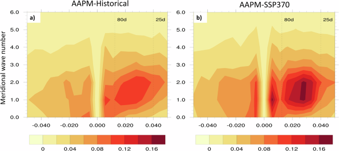
Space-time spectrum performed on daily precipitation anomalies for AAPM-Historical (a) and AAPM-SSP370 (b) over the region 10°S − 30°N and 80°E − 95°E. The X-axis represents frequency in day−1, and the Y-axis represents meridional wave number. The vertical dashed lines in each plot show the frequency corresponding to time periods of 25 days and 80 days.
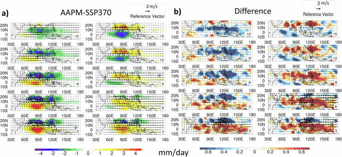
Propagation composite of AAPM-SSP370 projections for the time 2080–2099 (a), and the difference between AAPM-SSP370 and AAPM-Historical (b). Shading represents the ISO-filtered rainfall anomalies (mm/day) and vectors ISO-filtered winds at 850 hpa level (m/s). Only those values which are significant at 95% (using a two-tailed t-test) are shaded in (a)). The days relative to day 0 are printed in the bottom right of each plot, and reference vectors are printed on the top right of each panel. Note the difference in the reference vector between the left and right panels. Refer to Supplementary Fig. 15 for the scaled version of (b).
To understand why the spatiotemporal characteristics do not change in the SSP370 projections, we examine the background moisture and its gradients in the future projections with respect to the AAPM composite (Fig. 7). The background moisture increases uniformly throughout (Fig. 7c), except near and to the south of the equator (Fig. 7f), as evident from the difference with respect to AAPM composites. Hence, the meridional and zonal gradients remain the same in the future, and the equatorial convection on day 0 gets amplified and broadens relative to the historical run (Fig. 6). However, the static stability of the atmosphere is projected to increase in the future due to differential warming of the lower and upper troposphere42, which will lead to a very small change in the circulation response to the convective heating through the Weak Temperature Gradient (WTG) approximation43,44 (Fig. 7c). Thus, the moisture advection and its components remain mostly the same (Supplementary Fig. 6), leading to almost the same proportion of northward propagations and similar spatiotemporal characteristics in SSP370 projections. The ISO rainfall increases in future projections due to enhanced background moisture. On the day of maximum rainfall between 10°N − 20°N, we find that the ISO rainfall increases by 42% over the Arabian Sea (65°E − 75°E) and 63% over the Bay of Bengal (80°E − 95°E) compared to the historical runs. We also examined the propagation composites every 20 years (Supplementary Fig. 10) to find the rainfall increase consistently from 2020 to 2099.
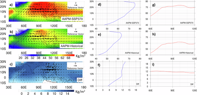
Background (JJAS mean) vertically integrated moisture (shading, kg/m2) and day 0 ISO wind anomaly at 850 hpa level (vectors, m/s) for AAPM-SSP370 (a) AAPM-Historical (b) and the difference between the two (c) (only values significant at 95% are shaded). Meridional structure of vertically integrated moisture in AAPM-SSP370 (d) AAPM-Historical (e) and the difference between the two (f) averaged over the longitudes 80°E − 95°E; the Y-axis represents latitude. Zonal structure of vertically integrated moisture for AAPM-SSP370 (g) AAPM-Historical (h) and difference (i) averaged over the latitudes 10°N − 20°N; the X-axis represents the longitude.
Figure 8 shows a schematic which summarizes the difference in propagation characteristics between the present and the future. With the increase in the moisture due to the warming of tropical Indian and Pacific oceans in the future, the excited Kelvin waves enhance the boundary layer convergence feedback45, leading to the amplification of BSISO precipitation and broadening of the region of convection in the zonal direction relative to the historical run46,47. However, these changes of broadening, along with the increased stability, oppose the effect of amplified convection, leading to a very subtle change in the wind perturbations. Thus, the moisture advection does not change substantially, leading to the same spatiotemporal characteristics of northward propagation. Nevertheless, the enhancement of background moisture enhances the BSISO rainfall as it moves northward from the equator.
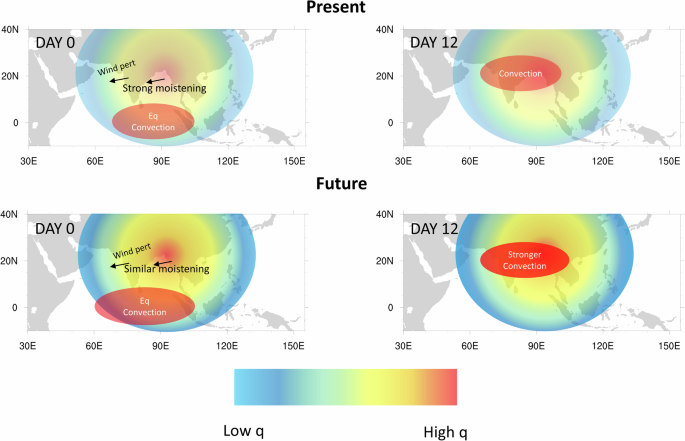
The multi-coloured shading represents the background moisture, and the red-coloured oval shape represents the convective centre. The shading intensity is representative of the strength. In the future climate, the background moisture will enhance uniformly throughout; thus, the background gradients remain the same. The day 0 equatorial convection is stronger and broader, leading to similar wind perturbations and, thus, similar moistening by the advection. Thus, the characteristics of northward propagation do not change. However, increased background moisture enhances the convection over the Bay of Bengal and Arabian Sea on day 12.
Discussion
In this study, we perform a moisture budget to understand why some CMIP6 models (BAPMs) do not robustly capture the northward propagating BSISO. The weaker horizontal advection is found to be responsible for this characteristic behaviour of BAPMs. This weaker horizontal advection is mainly caused by weaker wind perturbations and meridional gradient of moisture perturbation, which is a response of the atmosphere to equatorial convective heating. The BAPMs simulate weaker rainfall anomalies at the equator (Fig. 1b), leading to weaker wind and moisture perturbations, leading to weaker moisture advection and, thus, weaker northward propagation. In contrast, AAPMs, which simulate stronger equatorial convection, simulate robust northward propagation. Furthermore, the AAPM group also simulate a stronger eastward propagation of the ISO rainfall along the equator than the BAPM group.
Previous studies22,25 use the pattern correlation coefficient to distinguish a model’s ability to capture northward propagations, leading to a disparity between the models that would capture robust northward propagation and our AAPMs. However, the studies suggest that a model’s ability to simulate the vortex tilting distinguishes if a model could simulate the robust northward propagation or otherwise. In fact, even our AAPMs simulate a strong vortex tilting compared to the BAPMs (Supplementary Fig. 8). We find that the background zonal wind shear is not very different in the North Indian Ocean basin between AAPMs and BAPMs. Rather, the tilting is mainly controlled by the meridional gradient of vertical velocity ((frac{partial {omega }^{{prime} }}{partial y})). This gradient is mainly controlled by equatorial convective heating necessitated by the WTG balance, which is the dominant balance in the tropics48,49,50,51. The correlations between equatorial rainfall and (frac{partial {w}^{{prime} }}{partial y}) stand at 0.65 and 0.51 in the AAPMs and BAPMs, respectively (Supplementary Fig. 8c).
Finally, we use SSP370 projections to understand the fate of northward propagations in the future warming scenario. The proportion of northward propagations does not change substantially in the SSP370 projections due to the similar horizontal advection in the projections. However, the magnitude of BSISO rainfall increases by 42% in the Arabian Sea and 63% in the Bay of Bengal. The study implies that the large-scale BSISO environment becomes more conducive to bearing deeper convection, which could enhance the amplitude of extreme rainfall events associated with the BSISO in the future.
However, our study cannot address questions like “what magnitude of equatorial convection is required for the northward propagation in a fixed background zonal shear and moisture gradients?” and “what is the relative importance of the background zonal wind shear and the moisture gradients in the northward propagation?” A sensitivity study with a shallow water model with specified heating is warranted to answer these questions.
Data and methods
Data
We use CMIP6 historical data from 20 models (Table 1) to analyse BSISO’s northward propagation. We use the daily data of precipitation flux (pr), eastward wind (ua), northward wind (va), the Lagrangian tendency of pressure (wap), specific humidity (hus), and surface evaporation flux (hfls) (only taken from the available models). Most models have historical data from either 1850 or 1950 until 2014. Only the r1i1p1f1 variant is used in this study. Since Tropical Rainfall Measuring Mission’s (TRMM) precipitation data52, with which we intend to compare the CMIP6 data, is only available from 1998, we restrict ourselves to the time between 1998 and 2014 for the analysis presented. We also used ERA5 reanalysis data53 for winds and specific humidity to compare background states and characteristics of northward propagation. Data from all the models is re-gridded to a uniform 2.5° × 2.5° grid from its nominal resolution using area-conserving mapping.
Counting the northward propagations
In past works, authors used pattern correlation coefficients (PCC) on a Hovmöller plot to understand the model’s ability to capture the northward propagation or respective BSISO characteristics22,25,27. However, the PCC on the Hovmöller plots does not help understand the strength of ISO convection in the models. Moreover, they depend on the region we select to cluster events (Supplementary Fig. 1). Thus, in this work, we use a simple counting algorithm to count the northward propagation instead of PCC.
We first calculate daily anomalies from all the variables, followed by applying the Butterworth bandpass filter to extract the BSISO signal (ISO filtered from now on). Only 25–80 days (see Supplementary Fig. 7) periods are retained in the construction of filtered data. In our analysis, we only concentrate on the monsoon-time JJAS. The following algorithm counts the number of northward propagations from the equator in each model.
Algorithm 1
Counting the number of northward propagations
Step1: If the area averaged ISO-filtered rainfall over the region 5°S − 5°N, 80°E − 95°E is greater than the JJAS standard deviation of the ISO-filtered rainfall over the same region, the peak corresponding to that positive phase is taken as day 0.
Step 2: From day +5 to +20, we keep track of the ISO-filtered rainfall over the box 10°N − 20°N, 80°E − 95°E to the north of the initially chosen region. If, within this time, the ISO-filtered rainfall over this region crosses the JJAS standard deviation of ISO rainfall, then the event is counted as a northward propagating event.
Step 3: Repeat steps 1 and 2 for all the models in consideration.
Using the above algorithm, we find that the mean percentage of northward propagations for the model ensemble is 47% (Table 2). Hence, we label the models capturing over 47% of propagations as above-average-performing (AAPM) and under 47% of propagations as below-average-performing (BBPM) models. Thus, our analysis has 12 AAPMs and 8 BAPMs (Table 2). We then construct the composites of all the relevant variables in AAPMs and BBPMs to conduct the moisture budget. An example of how the above algorithm categorizes the events can be understood by examining Supplementary Fig. 12 (also refer to Supplementary Fig. 11 to understand the sensitivity of study to the size of model ensemble).
Moisture budget and decomposition of horizontal advection
The vertically integrated moisture budget equation scaled by the latent heat of vaporization is given by:
Where the prime terms represent the daily anomalies, Lv is the latent heat of vaporization, taken as a constant at 2.5 × 10⁶J/kg in this study. q is the specific humidity, V represents the horizontal velocity vector (u, v), which represents zonal velocity and meridional velocity respectively. ω is the pressure vertical velocity (Pa/s). P and E represent the precipitation flux and evaporation flux at the surface, respectively (kg/m2). Finally, 〈〉 represents the vertical integral of any operated quantity (mathop{int}nolimits_{1000}^{100}()dp/g). All the terms in Eq. (1) are ISO-filtered after they are constructed. The precipitation and vertical advection roughly balance each other, which can be seen by projecting each term onto precipitation in Eq. (1) (Supplementary Fig. 2), allowing us to define a term called columnar processes (({C}^{{prime} }))54,55 clubbing them together as:
This allows us to rewrite our equation as:
The moisture budget in this study is based on Eq. (3). The horizontal advection, which is the primary contributor to the moistening of the atmosphere ahead of the convection centre (Section “Results”), can be further split into zonal and meridional advection as:
To understand the processes responsible for the difference in propagations between AAPM and BAPM composites, we further break down the ISO-filtered zonal advection and meridional advection as:
Where the “–” terms represent the background state calculated as 80-day running mean, and the “({prime})” terms represent the deviation of any variable from the running mean (Note that “({prime})” terms in Eqs. (5) and (6) differ from Eq. (1) that in Eq. (1) the terms with “({prime})” were used to represent daily anomalies).
Projection
To understand the relative contributions of each term to the moisture tendency and the precipitation, we use the projections of all the terms in the budget (Eq. (4)). This projection of any term X onto the moisture tendency is obtained as54,55,56,57:
Where ∬dA represents the area-weighted integral. The projection onto precipitation can be obtained, replacing the moisture tendency term in Eq. (7) with precipitation (P).


Responses