Explainable AI reveals Clever Hans effects in unsupervised learning models

Main
Unsupervised learning is a subfield of machine learning (ML) that has gained prominence in recent years1,2,3. It addresses fundamental limitations of supervised learning, such as the lack of labels in the data or the high cost of acquiring them. Unsupervised learning has achieved successes in modelling the unknown, such as uncovering new cancer subtypes4,5 or extracting novel insights from large historical corpora6. Furthermore, the fact that unsupervised learning does not rely on task-specific labels makes it a good candidate for core artifical intelligence (AI) infrastructure: unsupervised anomaly detection provides the basis for various quality or integrity checks on the input data7,8,9,10. Unsupervised learning is also a key technology behind ‘foundation models’1,11,12,13,14,15, which extract representations upon which various downstream models (for example, classification, regression, ‘generative AI’ and so on) can be built.
The growing popularity of unsupervised learning models creates an urgent need to carefully examine how they arrive at their predictions. This is essential to ensure that potential flaws in the way these models process and represent the input data are not propagated to the many downstream supervised models that build upon them.
In this study, through conducting multiple investigations of popular unsupervised ML models of image data, we show that unsupervised learning models largely suffer from Clever Hans (CH) effects16. Specifically, we find that unsupervised learning models often produce representations from which instances can be correctly predicted to be, for example, similar or anomalous, although largely supported by data quality artefacts. The flawed prediction strategy is not detectable by common evaluation benchmarks such as cross-validation, but may manifest itself much later in ‘downstream’ applications in the form of unexpected errors, for example, if subtle changes in the input data occur after deployment (Fig. 1). While CH effects have been studied quite extensively for supervised learning16,17,18,19,20,21,22, the lack of similar studies in the context of unsupervised learning, together with the fact that unsupervised models supply many downstream applications, is a cause for concern.

The unsupervised model correctly predicts data instances as similar or anomalous, but does so using features that do not generalize well outside the available data. The CH effect typically goes undetected in a classical validation scheme and manifests itself in the form of prediction errors only after deployment. The problem is critical because the flaw can be inherited by potentially many downstream tasks. Our explainable AI approach allows CH effects to be detected directly in the unsupervised model and, in some cases, corrected. Pos, positive; pred, predicted; neg, negative. X-ray images reproduced from: left, middle, ref. 79 under a Creative Commons licence CC 1.0; right, ref. 90 under a Creative Commons licence CC BY-3.0.
For example, in image-based industrial inspection, which often relies on unsupervised anomaly detection9,10, we find that a CH decision strategy can systematically miss a wide range of manufacturing defects, resulting in potentially high costs. As another example, unsupervised foundation models of image data, advocated in the medical domain to provide robust features for various specialized diagnostic tasks, can potentially introduce CH effects into many of these tasks, with the prominent risk of large-scale misdiagnosis. These scenarios (illustrated in Fig. 1) highlight the practical implications of an unsupervised CH effect, which, unlike its supervised counterpart, may not be limited to malfunctioning in a single specific task, but potentially in all downstream tasks.
To uncover and understand unsupervised CH effects, we propose to use explainable AI23,24,25,26,27 (here techniques that build on the layer-wise relevance propagation (LRP) explanation framework28,29,30). Our proposed use of these techniques allows us to identify at scale which input features are used (or misused) by the unsupervised ML model, without having to formulate specific downstream tasks. We use an extension of LRP called BiLRP31 to reveal input patterns that are jointly responsible for similarity in the representation space. We also combine LRP with ‘virtual layers’32,33 to reveal pixel and frequency components that are jointly responsible for predicted anomalies.
Furthermore, our explainable AI-based analysis allows us to pinpoint more formal causes for the emergence of unsupervised CH effects. In particular, they are due not so much to the data, but to the unsupervised learning machine, which hinders the integration of the true task-supporting features into the model, even though vast amounts of data points are available. Our findings provide a novel direction for developing targeted strategies to mitigate CH effects and increase model robustness.
Overall, our work sheds light on the presence, prominence and distinctiveness of CH effects in unsupervised learning, calling for increased scrutiny of this essential component of modern AI systems.
Results
The CH effect can be defined as the property of a model to rely on features that are predictive in a particular setting (due to a spurious correlation between them and the true signal), but fail to remain so on new data, causing a significant drop in performance. (See also Supplementary Note D for a formal characterization and distinction from related concepts such as shortcut learning17 or human–AI alignment34,35.) Through experiments on two representative families of unsupervised models, representation learning and anomaly detection, and using explainable AI as our main analysis tool, we demonstrate the widespread presence of CH effects in unsupervised learning models, their adverse consequences and possible strategies to mitigate them.
CH effects in representation learning
We first investigate the CH effect in the context of using a recent medical foundation model to solve a COVID-19 detection task. Simulating an early pandemic phase characterized by data scarcity, we aggregate, similar to ref. 19, a large, well-established non-COVID-19 dataset with a more recent and smaller COVID-19 dataset. Specifically, we aggregate 2,597 instances of the National Institute of Health (NIH) CXR8 dataset36, collected between 1992 and 2015, with the 535 instances of the GitHub-hosted ‘COVID-19 image data collection’37, which contains COVID-19 instances from multiple sources. We refer to them as the ‘NIH’ and ‘GitHub’ subsets, respectively.
Further motivated by the need to accommodate the critically small number of COVID-19 instances and to avoid overfitting, we choose to rely on the representations provided by unsupervised foundation models15,38,39,40. Specifically, we feed our data into a pretrained PubMedCLIP model39, which has built its representation in an unsupervised manner from a very large collection of X-ray scans. On top of the PubMedCLIP model, we train a downstream classifier that separates COVID-19 from non-COVID-19 instances. It achieves a class-balanced accuracy of 87.5% on the test set (Table 1). However, a closer look at the structure of this performance score reveals a strong disparity between the NIH and GitHub subgroups, with all NIH instances being correctly classified and the GitHub instances having a lower class-balanced accuracy of 81.7%, and, more strikingly, a false positive rate (FPR) of 51%, as presented in Table 1. Considering that the higher heterogeneity of instances in the GitHub dataset is more characteristic of real-world conditions, this higher error estimate is more realistic. In particular, the high FPR of 51% precludes any practical use of the model in a hospitalization setting, where the model’s prediction should reliably and with low risk assist in the selection of appropriate medical treatment. We emphasize that this flaw in the model could have been easily overlooked if one had not paid close attention to (or known about) the data sources and instead relied only on the overall accuracy score.
To proactively detect this heterogeneous, non-robust prediction behaviour, we propose to use explainable AI. Specifically, to test whether the flaw has its sources in the unsupervised PubMedCLIP component, we use the BiLRP explanation technique31. BiLRP operates directly on similarity in the representation space without the need to formulate a specific downstream task. It is illustrated in Fig. 2 and its mathematical formulation is given in Methods. The output of BiLRP for two exemplary pairs of COVID-19-positive instances is shown in Fig. 3 (left). It shows that the modelled similarity comes from text-like annotations that appear in both images. This allows us to attribute the observed heterogeneity in performance to a CH effect and in turn to highlight broad risks for downstream applications (see Supplementary Note A for further analysis). We note that, unlike the per-group accuracy analysis above, our explainable AI analysis based on BiLRP did not require provenance metadata (GitHub or NIH) nor did it focus on a specific downstream task with its specific labels.
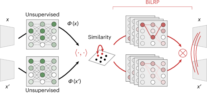
The output of BiLRP is a decomposition of the predicted similarity onto pairs of features from the two input images. It is typically displayed as a weighted bipartite graph connecting the contributing feature pairs.
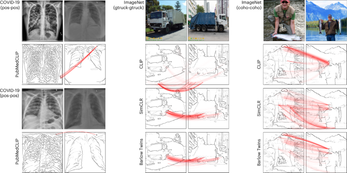
We show pairs of X-ray images from the GitHub subset, and pairs of natural images resembling ImageNet images from the classes garbage truck (gtruck) and coho, respectively. Explanations are generated using BiLRP. They highlight unexpected strategies used by the unsupervised models: for example, for X-ray data, similarity between instances arises from shared spurious textual annotations. For ImageNet data, similarity arises from logo artefacts or the presence of humans in the background. X-ray images reproduced from ref. 90 under a Creative Commons license CC BY-3.0. Credit: truck (left), Pixnio under a Creative Commons licence CC 1.0; truck (right), Pexels under a Creative Commons licence CC 1.0; fish (left), iStock.com/christiannafzger; fish (right), iStock.com/BrandyTaylor.
To test whether representation learning has a general tendency to evolve CH strategies beyond the above use case, we downloaded three generic foundation models, namely the original CLIP model13, SimCLR12,41 and Barlow Twins42. CLIP consists of an image encoder and a text encoder, and it aligns images to their associated text in representation space by minimizing a contrastive loss. SimCLR and Barlow Twins generate augmented views of the input image through random resized crops and colour augmentation, and maximize the similarity of these two views in representation space. As a downstream task, we consider the classification, using linear-softmax classifiers, of the 8 classes from ImageNet43 that share the WordNet ID ‘truck’ and of the 16 ImageNet classes that share the WordNet ID ‘fish’ (see Methods for details). The test accuracy of each model on these two tasks is given in Table 1 (columns ‘original’). On the truck classification task, the CLIP model performs best, with an accuracy of 84.7%. On the fish classification task, the CLIP and supervised models perform best, with accuracies of 85.4% and 85.9%, respectively.
We use BiLRP to examine the representations of these unsupervised models. In Fig. 3 (centre), we observe that CLIP-based similarities, as in PubMedCLIP, also rely on text. Here, a textual logo in the lower-left corner of two garbage truck images is used to support the similarity, suggesting a CH effect (see ref. 20 for a similar finding in supervised learning). SimCLR and Barlow Twins ignore the text and rely instead on the actual garbage truck. In the fish classification task (Fig. 3, right), we observe that all unsupervised models amplify humans over fish features, again suggesting a CH effect.
To establish the CH nature of the logo and human detection strategies identified by BiLRP, we proceed to test the models on specific data subgroups that may be more prevalent under operational conditions. The results are presented in Table 1. We observe a systematic degradation in performance when moving from the original data to some of these data subsets. For example, when we break the spurious correlation between logo and truck class by inserting a logo on each truck image, we observe a drop in the accuracy of the CLIP model from 84.7% to 80.3% (column ‘logo’ in Table 1). Sharper drops in performance can be observed when looking at individual classes, such as tow trucks, which are generally difficult to separate from garbage trucks (Supplementary Note B). For the fish case, a similar drop in accuracy is observed for SimCLR and Barlow Twins from 81.4% and 83.2% to 74.8% and 75.8%, respectively, when only images containing humans are retained and class rebalancing is performed. In the case of CLIP, its lack of focus on fish is surprisingly not associated with a similar drop in performance, leaving open the question of what exact strategy allows CLIP to generalize well on this data. A detailed analysis of the structure of the prediction errors for each model and classification task, supported by confusion matrices, is given in Supplementary Note B.
To better assess the risk of CH effects in unsupervised learning, it is necessary to reflect on the more abstract factors that contribute to their occurrence. The heterogeneity of strategies revealed by BiLRP for models otherwise trained on similar large datasets suggests that the unsupervised learning machine, more than the data, is crucial in shaping the data representation strategy. In the case of SimCLR and Barlow Twins, the systematic amplification of humans in the centre of the image can be attributed to their random crop matching objective, where those features in the centre of the image carry the most mutual information across random crops (for further studies of amplification/suppression effects in these models, we refer to refs. 44,45,46,47). When considering the CLIP and PubMedCLIP models, the systematic amplification of textual logos, faces or other identifying features can be attributed to their image–text matching objective, which tends to amplify any features from the two modalities that carry mutual information.
In summary, while the matching tasks defined in, for example, CLIP, SimCLR and Barlow Twins intuitively aim to introduce useful prior knowledge and invariance into the representation, they can, on certain data subsets, lead to strong imbalances in the expression of different features. These imbalances are prone to cause CH effects and, in turn, loss of accuracy in downstream tasks.
CH effects in anomaly detection
Extending our investigation of the CH effect to another area of unsupervised learning, namely anomaly detection, we consider an industrial inspection use case based on the popular MVTec-AD dataset9. The dataset consists of 15 product categories, each consisting of a training set of images without manufacturing defects and a test set of images with and without defects. Since manufacturing defects are infrequent and heterogeneous in nature, the problem is typically approached using unsupervised anomaly detection2,9. These models map each instance to an anomaly score, from which threshold-based downstream models can be built to classify between instances with and without manufacturing defects. Unsupervised anomaly detection has received considerable attention, with sophisticated approaches based on deep neural networks such as PatchCore48 or EfficientAD49 showing excellent performance in detecting a wide range of industrial defects.
Somewhat surprisingly, simpler approaches based on distances in pixel space show competitive performance for selected tasks2. We consider one such approach, which we call ‘D2Neighbors’, where anomalies are predicted according to the distance to neighbours in the training data. Specifically, the anomaly score of a new instance x is computed as f(x) = softminj{∥x − uj∥2} where ({({{{bf{u}}}}_{j})}_{i = 1}^{N}) is the set of available inlier instances (see Methods for details on the model and data preprocessing). This anomaly model belongs to the broader class of distance-based models50,51,52, and connections can be made to kernel density estimation53,54 and one-class support vector machines55. Using D2Neighbors, we are able to build downstream models that classify industrial defects of the MVTec data with F1 scores above 0.9 for five categories (bottle, capsule, pill, toothbrush and wood).
To shed light on the prediction strategy associated with these unexpectedly high F1 scores, we make use of explainable AI. Specifically, we consider an extension of LRP for anomaly detection30,56 and further equip the explanation technique with ‘virtual layers’32,33. The technique of ‘virtual layers’ (Fig. 4) is to map the input to an abstract domain and back, leaving the prediction function unchanged, but providing a new representation in terms of which the prediction can be explained. We construct such a layer by applying the discrete cosine transform (DCT)57, shown in Fig. 4 (bottom right), followed by its inverse. This allows us to explain the predictions jointly in terms of pixels and frequencies.
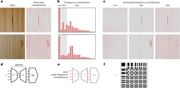
a, Images synthesized to resemble MVTec-AD (class wood) and pixel-wise LRP explanations of the anomaly predictions. The explanations for other MVTec-AD categories are given in Supplementary Note C. b, Frequency domain explanations. The x axis represents the frequencies (on a power scale) and the y axis is the contribution of the corresponding frequencies to the anomaly prediction. c, Pixel-wise contributions filtered by frequency band. d, A schematic of the virtual inspection layer used to explain anomalies in the joint pixel-frequency domain. e, Pixel-wise contributions are filtered by blocking frequency contributions within the virtual layer. f, The basis elements of the DCT, which we use to map pixels to frequencies and back.
The result of our proposed analysis is shown in Fig. 4 for two wood instances (see Supplementary Note C for instances of different categories). Explanations at the pixel level show that D2Neighbors supports its anomaly predictions largely based on pixels containing the actual industrial defect. The squared difference in its distance function ((parallel varDelta {parallel }^{2}={sum }_{i}{varDelta }_{i}^{2})) encourages a sparse pixel-wise response of the model, efficiently discarding regions of the image where the new instance shows no difference from instances in the training data. However, we also see in the pixel-wise explanation that a non-negligible part of the anomaly prediction comes from irrelevant background pixels. Joint pixel-frequency explanations shed light on these unresolved contributions, showing that they arise mostly from the high-frequency part of the model’s decision strategy (Fig. 4b,c).
The high exposure of the D2Neighbors model to these irrelevant high-frequency features, as detected by our LRP analysis, raises the suspicion that we are again in the presence of a CH effect. We simulate an innocuous postdeployment perturbation of the data preprocessing by changing the image resizing algorithm from OpenCV’s nearest neighbour resizing to a more sophisticated resizing method that includes antialiasing, a procedure that cuts high frequencies to eliminate resizing artefacts. In practice, such a change may result from a software update, for example. Resizing techniques have been shown in some cases to substantially affect image quality and image generation metrics58, but their effect on general ML models, especially unsupervised ones, has been little studied. The performance of the D2Neighbors model before and after changing the resizing algorithm is presented in Table 2 (columns ‘original’ and ‘deployed’, respectively). The F1 score performance of D2Neighbors degrades by almost 10 percentage points. This performance degradation, along with D2Neighbors’ reliance on high frequencies revealed by LRP, exposes the CH nature of the model: when antialiasing is introduced into the resizing procedure, the high frequencies that the D2Neighbors model uses to support its prediction disappear from the data, significantly reducing each instance’s anomaly score and causing the performance degradation. This performance degradation of D2Neighbors under postdeployment conditions is particularly surprising given that the data quality has actually improved. Looking more closely at the structure of the performance degradation, we see that the false negative rate (FNR) rises sharply from 4% to 23% (Table 2), which can be explained by the absence of anomaly-contributing high frequencies after deployment. In an industrial inspection setting, an increase in FNR can have serious consequences, in particular, many defective instances may be missed and propagated through the production chain. This can result in wasted resources in subsequent production stages and high recall costs.
As in the case of representation learning, it is useful to ask what factors contribute to the CH effect. We trace the D2Neighbors CH strategy to the distance functions it relies on. Unlike the linear layers commonly used in supervised learning, distances cannot inherently build invariance to specific directions in the input space, exposing models to a manifold of irrelevant data perturbations. Despite this tendency to overexposure, distance functions (including the usual Euclidean distance as well as ℓp variants) are a building block of many popular unsupervised anomaly models, their primary advantage being that they generate a decision boundary without requiring a representative set of anomalous instances to contrast against. Distance functions also appear in the more advanced PatchCore model48 where they are computed on top of more abstract visual features (Methods). As presented in Table 2, they also suffer a significant drop in performance after deployment, suggesting that they are affected by a similar CH effect. Overall, our analysis highlights the challenge of creating anomaly models that are both general enough not to miss unexpected anomalies, but also not overexposed so as not to increase the risk of CH effects.
Alleviating CH in unsupervised learning
Leveraging the explainable AI analysis above, we aim to build models that are more robust across different data subgroups and in postdeployment conditions. Unlike previously proposed CH removal techniques20,21, we aim to operate on the unsupervised model rather than the downstream tasks. This allows us to potentially achieve broad robustness improvements while leaving the downstream learning machines (training supervised classifiers or adjusting detection thresholds) untouched. We first consider the CLIP model, which our explainable AI analysis has shown to incorrectly rely on text logos, and proceed by removing CLIP activations whose response differs most between images of the logo and non-logo subgroups (details in Methods). We also experiment with a CH mitigation approach for anomaly detection, where we prune the high frequencies spuriously used by the model by inserting a blur layer at the input of the model (details in Methods). In both cases, the proposed CH mitigation technique improves model robustness, largely reversing the performance degradation observed in simulated postdeployment conditions (Tables 1 and 2, rows ‘CH mitigation’). Our CH mitigation experiments, which effectively modify the structure of the model, again underscore the primary role of the learning machine in allowing or preventing CH effects.
Discussion
Unsupervised learning is an essential category of ML that is increasingly being used in core AI infrastructure to power a variety of downstream tasks, including classification, regression and also ‘generative AI’. Much research so far has focused on improving the performance of unsupervised learning algorithms, for example, to maximize downstream classification accuracy. These evaluations often pay little attention to the exact strategy used by the unsupervised model to achieve the reported high performance, in particular whether these models rely on CH strategies.
Using advanced explainable AI techniques such as BiLRP or LRP in the frequency domain, we have shown that CH strategies are widespread in unsupervised learning. These strategies can take several forms, such as predicting correctly but based on features such as text that are spuriously amplified in the unsupervised representation, or based on high-frequency features to which unsupervised anomaly models are overexposed. These flawed prediction strategies no longer work well when the data distribution changes after deployment. As shown in two use cases, this can have important practical consequences such as widespread misdiagnosis of patients or systematic failure to recall manufacturing defects. Importantly, the same flawed unsupervised representation can produce CH effects in any of its potentially many downstream models.
Addressing these CH effects is therefore crucial to apply unsupervised learning more reliably. However, compared with CH effects in supervised learning, another dimension of complexity is added to the problem: one has to decide whether to handle CH effects in the downstream models or directly in the unsupervised model part. Revising downstream models (for example, with human feedback20,21,59 or in response to changing conditions60,61,62,63) may help to maintain high accuracy on the given task. However, it is not sustainable if we consider that the procedure would have to be repeated for every single downstream task. This may be necessary even after a flaw in the foundation model becomes known (for example, refs. 64,65) since building a new unsupervised model is computationally expensive and requires extensive testing. Instead, we have proposed in this paper to address CH effects directly in the design of the unsupervised model, with the goal of achieving persistent robustness that benefits all existing and future downstream applications.
However, this requires a better formal understanding of the reasons for CH effects in unsupervised learning. We found that they differ substantially from those in supervised learning in that they arise less from data quality issues and more from flaws in the design of the unsupervised learning machine. For example, our study showed that unsupervised anomaly detection is structurally unable to reduce its exposure to high frequencies and thus also fails to reproduce common filtering mechanisms found in supervised learning66,67,68, with D2Neighbors being a prominent example. The high risk of generalization error caused by feature overexposure led us to ask the more fundamental question of ‘what are appropriate model selection criteria for unsupervised learning’. D2Neighbors, with its apparent simplicity, would probably fare well under Occam’s razor or other classical model selection criteria, although our experiments have shown that it clearly lacks generalizability and robustness. Thus, it seems essential to refine these criteria to include overexposure or feature balancing as additional factors.
Having shed light on reasons for the emergence of CH effects in unsupervised learning, we have experimented with CH mitigation strategies based on feature rebalancing or exposure reduction, and have been able to achieve performance improvements on difficult data subgroups or in simulated postdeployment conditions. In doing so, we have demonstrated the actionability of our analysis, showing that it can guide the process of identifying and subsequently correcting the faulty components of an unsupervised learning model.
While our investigation of unsupervised CH effects and their consequences has focused on image data, extension to other data modalities seems straightforward. Explainable AI techniques such as LRP operate independently of the type of input data. LRP has recently been extended to recurrent neural networks69, graph neural networks70, transformers71 and state space models72, which represent the state of the art for large language models and other models of structured data. Thus, our analysis could be extended in the future to analyse other instances of unsupervised learning, such as anomaly detection in time series or the representations learned by large language models (for example, refs. 73,74).
Overall, through the application of recent explainable AI techniques, our work has contributed to highlighting the pervasiveness of CH effects in unsupervised learning, the multiple factors that lead to them, the resulting loss of accuracy on new data and possible ways to mitigate these CH effects. We believe that the CH effect in unsupervised learning, and the uncontrolled risks associated with it, is a question of general importance, and that explainable AI and its recent developments provide an effective way to tackle it.
Methods
This section first introduces the unsupervised ML models studied in this work, the datasets on which they are applied and the considered CH mitigation techniques. It then presents the LRP method for explaining predictions, its BiLRP extension for explaining similarity and the technique of ‘virtual layers’ for generating joint pixel-frequency explanations.
ML models and data for representation learning
Representation learning experiments were performed on the PubMedCLIP39, CLIP13, SimCLR12,41 and Barlow Twins42 models. PubMedCLIP is a representation learning model specialized for X-ray data. It is based on a pretrained CLIP model (described below) and fine tuned on the ROCO dataset75, a collection of radiology and image caption pairs. In our experiments, we chose the variant based on the ResNet-50 architecture and downloaded the weights from ref. 76. CLIP learns representations using a large collection of image–text pairs from the internet. Images are given to an image encoder and the corresponding texts are given to a text encoder. The similarity of the two resulting embeddings is then maximized with a contrastive loss. In our experiments, we again chose the ResNet-50 variant with weights from ref. 77. SimCLR augments the input images with resized crops, colour jitter and Gaussian blur to create two different views of the same image. These views are then used to create positive and negative pairs, where the positive pairs represent the same image from two different perspectives and the negative pairs are created by pairing different images. The contrastive loss objective maximizes the similarity between the representations of the positive pairs while minimizing the similarity between the representations of the negative pairs. In our experiments, we used the ResNet-50 architecture and weights from the vissl library (https://vissl.ai/). Barlow Twins is similar to SimCLR in that it also generates augmented views of the input image through randomly resized crops and colour augmentation, and maximizes their similarity in representation space. However, it differs from SimCLR in the exact mechanisms used to prevent representation collapse. In our experiments, we again used the ResNet-50 architecture and took the weights from ref. 78. For our representation learning experiments, we also considered a supervised baseline, with the same ResNet-50 architecture, but trained in a purely supervised fashion using backpropagation. We used the default model weights from the torchvision library.
Downstream classifiers
To establish the CH effect in these unsupervised models, specifically its manifestation in downstream tasks, we built linear classifiers (readouts) on top of the unsupervised representations. For binary detection tasks, specifically detection of COVID-19 instances, we trained a linear support vector machine classifier (details in Supplementary Note A), with the slack parameter C set to 0.01 through a hold-out validation procedure. For multiclass classification problems (classifying among the 8 types of trucks and among the 16 types of fishes), we instead used a logistic regression classifier (sklearn) with the lbfgs solver, l2 regularization (C = 1.0), no bias term, a maximum of 1,000 iteration steps and class-balanced sampling.
Datasets
The analysis and training of these models were performed on different datasets. For the X-ray experiments, we combined the NIH ChestX-ray8 (CXR8) dataset36,79 and the GitHub-hosted ‘COVID-19 image data collection’37,80. The GitHub dataset contains 342 COVID-19-positive and 193 COVID-19-negative images. We split the data 80:20 into training and test sets. This resulted in 272 positive and 168 negative images in the training set and 70 positive and 25 negative images in the test set. The training split was consolidated by adding 2,552 randomly selected negative images from the NIH dataset. We also expanded the test set by adding another 45 randomly selected negative images from NIH to obtain a class-balanced test set. The selection was made so that the same patient IDs did not appear in both the training and test sets. All images were resized and centre-cropped to 224 × 224 pixels. The ImageNet experiments were performed on two ImageNet subsets. First, the ‘truck’ subset, consisting of the eight classes sharing the WordNet ID ‘truck’ (minivan, moving van, police van, fire engine, garbage truck, pickup, tow truck and trailer truck), resulting in a dataset of 10,259 training and 400 test examples. Then the ‘fish’ subset, consisting of the 16 classes sharing the WordNet ID ‘fish’ (tench, barracouta, coho, sturgeon, gar, stingray, great white shark, hammerhead, tiger shark, puffer, electric ray, goldfish, eel, anemone fish, rock beauty and lionfish), resulting in 20,334 training and 800 test examples.
ML models and data for anomaly detection
The D2Neighbors model used in our experiments is an instance of the family of distance-based anomaly detectors, which encompasses a variety of methods from the literature2,50,51,52,81,82. The D2Neighbors model computes anomaly scores as (o({{bf{x}}})={{mathbb{M}}}_{j}^{gamma }left{parallel {{bf{x}}}-{{{bf{u}}}}_{j}{parallel }_{p}^{p}right}) where x is the input, ({({{{bf{u}}}}_{j})}_{j = 1}^{N}) are the training data and ({{mathbb{M}}}^{gamma }) is a generalized f-mean, with (f(t)=exp (-gamma t)). The predicted anomaly scores can be interpreted as a soft minimum over distances to data points, that is, a distance to the nearest neighbours. In our experiments, the data received as input are images of size 224 × 224 with pixel values encoded between −1 and 1, downsized from their original high resolution using OpenCV’s fast nearest neighbour interpolation. We set γ so that the average perplexity83 equals 25% of the training set size for each model.
We also considered the PatchCore48 anomaly detection model, which uses mid-level patch features from a fixed pretrained network. It constructs a memory bank of these features from nominal example images during training. Anomaly scores for test images are computed by finding the maximum distance between each test patch feature and its nearest neighbour in the memory bank. Distances are computed between patch features ϕp(x) and a memory bank of location-independent prototypes ({({{{bf{u}}}}_{j})}_{j = 1}^{N}). The overall outlier scoring function of PatchCore can be written as (o({{bf{x}}})={max }_{k}{min }_{j}parallel {phi }_{k}({{bf{x}}})-{{{bf{u}}}}_{j}parallel). The function ϕk is the feature representation aggregated from two consecutive layers at spatial patch location k, extracted from a pretrained WideResNet50. The features from consecutive layers are aggregated by rescaling and concatenating the feature maps. The difference between our reported F1 scores and those in ref. 48 is mainly due to the method used to resize the images. We used the authors’ reference implementation84 as the basis for our experiments.
Datasets
All models above were trained on the MVTec-AD dataset. The MVTec-AD dataset consists of 15 image categories (‘bottle’, ‘cable’, ‘capsule‘, ’carpet’, ‘grid’, ‘hazelnut’, ‘leather’, ‘metal nut’, ‘pill’, ‘screw’, ‘tile’, ‘toothbrush’, ‘transistor’, ‘wood’ and ‘zipper’) of industrial objects and textures, with good and defective instances for each category. For the experiments based on D2Neighbors, we simulated different data preprocessing conditions before and after deployment by changing the way images are resized from their original high resolution to 224 × 224 pixels. We first used a resizing algorithm found in OpenCV v.4.9.0 (ref. 85) that is based on nearest neighbour interpolation. We then simulated postdeployment conditions using an improved resizing method, specifically a bilinear interpolation implemented in Pillow v.10.3.0 and used by default in torchvision v.0.17.2 (ref. 86). This improved resizing method includes antialiasing, which has the effect of smoothing the transitions between adjacent pixels of the resized image.
Details of CH mitigation techniques
We describe in detail the CH mitigation techniques we use to mitigate the reliance of ML models on spurious features. To prune textual logos in the CLIP model, we computed responsiveness by measuring the difference in activation between a set of randomly selected truck images with and without a watermark logo, and then pruning (that is, setting to zero) the top k filters in the bottom of the image (we pruned five such filters in the main paper and experimented with different values of k in the Supplementary Information). We looked at multiple layers, and chose an early layer of the CLIP model (encoder.relu3) as it showed a large difference on just a few filters compared to more abstract layers later in the network. In our anomaly detection experiments, where our analysis revealed a spurious use of high frequencies, we proposed to address the CH effect by pruning those high frequencies, specifically by adding a low-pass filter at the input of the model, which convolves the red, green and blue channels individually with Gaussian filters of size 11 × 11.
Explanations for representation learning
Our experiments examined dot product similarities in representation space, that is, (y=langle {boldsymbol{Phi}} ({{bf{x}}}),{boldsymbol{Phi}} ({{bf{x}}}^{prime} )rangle), where Φ denotes the function that maps the input features to the representation, typically a deep neural network. To explain similarity scores in terms of input features, we used the BiLRP technique31 which extends the LRP technique26,28,29,87 for this specific purpose. The conceptual starting point of BiLRP is the observation that a dot product is a bilinear function of its input. BiLRP then proceeds by reverse propagating the terms of the bilinear function to pairs of activations from the layer below and iterating down to the input. Denoting by ({R}_{k{k}^{{prime} }}) the contribution of neurons k and ({k}^{{prime} }) to the similarity score in some intermediate layer in the network, BiLRP extracts the contributions of pairs of neurons j and ({j}^{{prime} }) in the layer below via the propagation rule
In this formula, zjk denotes the contribution of neuron j to the activation of neuron k. In practice, the reverse propagation procedure above can be implemented equivalently, but more efficiently and easily, by computing a collection of standard LRP explanations (one for each neuron in the representation layer) and recombining them in a multiplicative manner
Overall, assuming the input consists of d features, BiLRP produces an explanation of size d × d, which is typically represented as a weighted bipartite graph between the set of features of the two input images. Due to the large number of terms, pixel-to-pixel contributions are aggregated into patch-to-patch contributions, and elements of the BiLRP explanations that are close to zero are omitted in the final explanation rendering. In our experiments, we computed BiLRP explanations using the Zennit implementation of LRP88, which handles the ResNet-50 architecture, and set Zennit’s LRP parameters to their default values.
Explanations for the D2Neighbors model
The D2Neighbors model we investigate for anomaly detection is a composition of a distance layer and a soft min-pooling layer. To handle these layers, we use the purposely designed LRP rules of refs. 30,56. Propagation in the softmin layer (({{mathbb{M}}}_{j}^{gamma })) is given by the formula
a ‘min-take-most’ redistribution, where f is the same function as in ({{mathbb{M}}}_{j}^{gamma }). Each score Rj can be interpreted as the contribution of the training point uj to the anomaly of x. To further propagate these scores into the pixel-frequency domain, we adopt the framework of ‘virtual layers’32,33 and adapt it to the D2Neighbors model. As a frequency basis, we use the DCT57, shown in Fig. 4 (bottom right), which we denote by its collection of basis elements ({({{bf{v}}}_{k})}_{k}). Since the DCT forms an orthogonal basis, we have the property ({sum }_{k}{{bf{v}}}_{k}{{{bf{v}}}}_{k}^{top }=I), and multiplication by the identity matrix can be interpreted as a mapping to the frequencies and back. For the special case where p = 2, the distance terms in D2Neighbors reduce to the squared Euclidean norm ∥x − uj∥2. These terms can be developed to identify pixel–pixel-frequency interactions: (parallel {{bf{x}}}-{{{bf{u}}}}_{j}{parallel }^{2}={({{bf{x}}}-{{{bf{u}}}}_{j})}^{top }({sum }_{k}{{{bf{v}}}}_{k}{{{bf{v}}}}_{k}^{top })({{bf{x}}}-{{{bf{u}}}}_{j})) (={sum }_{k}{sum }_{i{i}^{{prime} }}{[{{bf{x}}}-{{{bf{u}}}}_{j}]}_{i}{[{{bf{x}}}-{{{bf{u}}}}_{j}]}_{{i}^{{prime} }}{[{{{bf{v}}}}_{k}]}_{i}{[{{{bf{v}}}}_{k}]}_{{i}^{{prime} }}). From there, one can construct an LRP rule that propagates the instance-wise relevance Rj to the pixel–pixel-frequency features:
where the variable ϵ is a small positive term that handles the case where x and uj overlap. A reduction of this propagation rule can be obtained by marginalizing over interacting pixels (({R}_{ik}={sum }_{{i}^{{prime} }}{R}_{i{i}^{{prime} }k})). Further reductions can be obtained by marginalizing over pixels (Rk = ∑iRik) or frequencies (Ri = ∑kRik). These reductions are used to generate the heat maps in Fig. 4.
Reporting summary
Further information on research design is available in the Nature Portfolio Reporting Summary linked to this article.
Responses