Exposing hidden periodic orbits in scanning force microscopy
Introduction
Control of nanomechanical dynamics is of extreme technological importance. Applications range from motion and position sensors1, detection of chemical and biological species2,3,4, transducers and microfluidic transport5, to more fundamental demands such as gravitational wave detection and quantum state analysis6,7,8. Typically, the resulting dynamics are treated linearly, i.e., in terms of a driven, damped harmonic oscillator, where a stationary state corresponds to a periodic orbit. As for any oscillator, however, increasingly nonlinear external forces result in drastic changes in the frequency response, up to the emergence of bifurcation points or even chaotic behavior9,10,11,12,13,14,15,16,17,18,19,20. For micro-cantilevers in the vicinity of a surface, the nonlinearity can originate from repulsive (i.e., hardening), attractive (i.e., softening), or combined interaction9,21,22. As a result, multiple branches of stable states emerge23,24, and the system may change quasi-erratically between them, triggered by external disturbances such as varying ambient conditions or noise.
These stable states are separated by unstable states, which, however, are experimentally not directly accessible because of their unstable character: infinitesimal deviations from the ideal stationary point in Fourier space rapidly drive the oscillator toward one of the stable solutions. Experimental access to unstable states has been realized via control-based continuation methods for macroscopic mechanical systems25,26,27,28,29, and via phase control for miniaturized oscillators30, offering a variety of advantages over the uncontrolled system, such as an extended parameter space for reliable operation, or improved noise performance and hence resolution31. The first attempts to apply control-based continuation methods to atomic force microscopy can be found in ref. 32. However, the proposed method was only tested in a simulation of a model.
In this work, we explore nonlinear surface-engaged nanomechanical oscillators as they are employed in dynamic scanning force microscopy (SFM), particularly the concept of stabilizing an unstable branch of periodic orbits of an SFM cantilever in the vicinity of a solid sample surface. Scanning force microscopy, also known as atomic force microscope (AFM), is a versatile and popular method for revealing surface properties on the nanoscale. These include morphology, atomic and molecular structure, stiffness, surface potential, magnetic field, and many more33,34. Material parameters can be extracted, e.g., employing phase imaging, force-distance curves34, multimodal SFM35, or by analyzing transient deflection data 36, e.g., by using sparse identification of nonlinear dynamics (SINDy) 37. Application scenarios of SFM in the past decades range from atomic and molecular systems to life-sciences34,38,39,40. In short, in this method, a sharp tip attached to a microcantilever beam is approached to the sample surface. The resulting beam deflection due to tip-sample interaction is measured and processed further, usually in a closed-loop manner. Most SFM modes rely on the periodic mechanical actuation of the cantilever on one of its eigenmodes, where continuous changes of the periodic orbits are indicative of varying sample properties, e.g., as a function of the lateral position of the tip.
While usually treated as a harmonic oscillator, tip-sample interaction forces are highly nonlinear, hence the SFM represents a prototype nanomechanical system. However, transferring control concepts to the SFM is not straightforward, for both technical and physical reasons: when interacting with a surface, the attractive van-der-Waals interaction dominates all other forces41, if not the even larger capillary forces come into play, e.g., due to condensation of a water meniscus. Therefore, the relevant external forces acting on the oscillator are fundamentally different compared to macroscopic or intrinsically nonlinear systems, and the same holds for the shape of frequency-response curves34. Since the tip-sample distance critically affects the oscillator’s properties on the nano- or even atomic scale, stable and precise distance control is crucial. In this work, we are aiming at stabilizing unstable states of a conventional SFM with nanometer amplitudes, while leaving the system’s intrinsic properties unchanged via non-invasive control-based continuation42. As a useful side effect, unwanted sudden jumps between temporarily stable periodic orbits can be avoided, leading to further robustness of SFM measurements, which otherwise has to be actively enforced using dedicated approaches43.
Results and discussion
Bifurcation diagram of a nonlinear oscillator
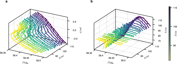
Figure 1 shows a typical bifurcation diagram of a nonlinear oscillator with an attractive (i.e., softening) external force. A natural set of independent parameters for an SFM consists of the driving frequency f and the (mean) tip-sample separation s, which both serve as bifurcation parameters in our setup. The latter adjusts the strength of the external nonlinear force. The state can be characterized by the cantilever’s amplitude A(f) (Fig. 1a and phase ϕ(f) of the deflection with respect to the driving frequency (Fig. 1b), although other descriptors may be appropriate as well, such as a complex Fourier vector28. Starting far away from the sample (i.e. large s), the frequency-response A(f) resembles that of a typical driven, damped harmonic oscillator with its maximum at the resonance frequency f0. As the nonlinearity increases (i.e. s decreases), the resonance initially shifts, then deforms, until it finally enters the bistable regime where A is not uniquely determined by f: for a given frequency f, there are two stable periodic orbits separated by an unstable one. In a pseudo-3D representation (Fig. 1), the set of amplitudes or phases of stationary states in Fourier space describes a folded surface, respectively.
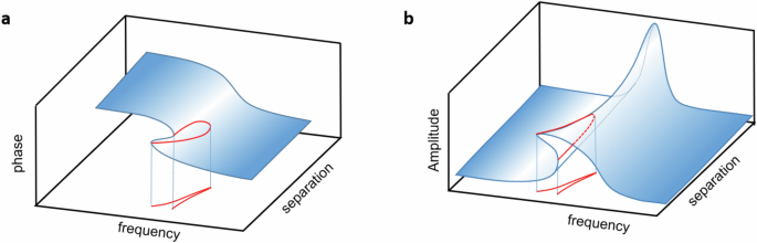
a amplitude A and b phase ϕ of a surface-engaged nano-oscillator under attractive interaction. The red lines indicate positions of bifurcation points and their projection onto the separation-frequency plane.
In experimental frequency sweeps, the bistability manifests as sudden amplitude jumps, also called catastrophes, accompanied by a pronounced hysteresis behavior (Fig. 2a. The resulting shape of A(f) is occasionally referred to as shark fin, where the orientation of the shark fin depends on the sign of the nonlinear force. The branches of unstable states extend within the region between the two bifurcation points (red curve indicated in Fig. 1a and cover a considerable part of the amplitude range. At the smallest separation (s ≈ 61 nm in Fig. 2a), the shark fin appears to point to both directions, left and right, for the frequency down-sweep, as well as for the up-sweep.
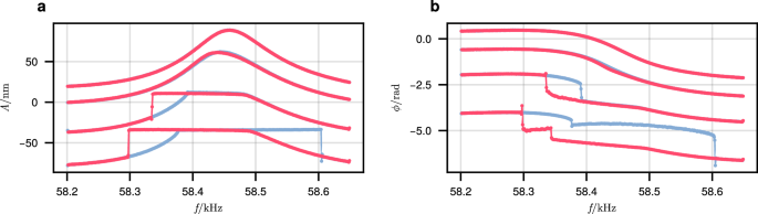
a Amplitude A and b phase ϕ on a silicon sample for various separations s, ranging from a free oscillation (largest separation, top), to slightly attractive, attractive, and coexisting attractive and repulsive (lowest separation, bottom) forces. Red curves indicate sweeps from high to low frequencies and blue curves from low to high. The curves are offset vertically by an arbitrary amount for clarity.
This is a consequence of the coexistence of attractive and repulsive forces, resulting in a complex double-bent frequency-response curve34. Some of the bifurcation points are hardly visible, because the sudden amplitude change is small, e.g., for the forward sweep (blue curves). However, the same bifurcation points are also formed in the phase response (Fig. 2b), where they are clearly visible. The unstable part of the fold in Fig. 1a, b is inaccessible by simple frequency sweeps. In the following we present a method enabling measurement of such hidden folds of the response surface in SFM experiments.
Tracking unstable states
Our mathematical and experimental approach is summarized graphically in Fig. 3 and described in detail in the Methods section. In short, the tip of an SFM is approached to a silicon sample, and a periodic force is applied to the cantilever. The phase of the first Fourier component of the resulting oscillation state is extracted and used as an input parameter for a non-invasive control scheme, implemented in a real-time signal processing unit (RTSPU). The control acts on the frequency (f=frac{1}{2pi }frac{{{{rm{d}}}}}{{{{rm{d}}}}t}psi), which results in a time-dependent forcing signal of the form (Gamma sin (psi (t))), where the accumulated phase ψ(t) (often referred to as instantaneous phase) is obtained by integrating the proportional plus integral controller
with initial conditions ψ(0) = 0 and λ(0) = 0, a starting angular frequency ωs, the target phase ϕ⋆, the integral part λ, and control gains KP, KI. Note that this control law is non-invasive by design44, in that it does not alter the system’s dynamics once the control target is reached. Instead of the commonly utilized lock-in amplifier for phase extraction, we implemented a successive phase detector based on the normalized least-mean-square (nLMS) method45, which turned out to be an essential ingredient due to its superior rate of convergence46. Once a stationary point in Fourier space is reached with sufficient accuracy, a new control step is started where the target phase is decremented by a constant value, such that the entire relevant phase range is sampled in both, stable and unstable regions. Then, the tip-sample separation is changed such that the full set of periodic orbits is tracked while still residing in the predominantly attractive regime of the tip-surface interaction. Hence, double-bent bifurcation diagrams, as described in the previous section, are largely avoided for simplicity.
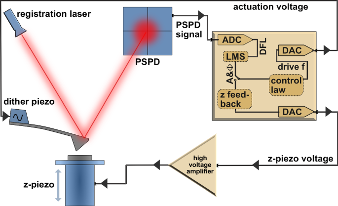
Blue-colored parts symbolize parts of the commercial SFM setup, beige components were added later on and integrated via a breakout-box. As the z-piezo voltage is kept constant during control attempts, the tip-sample distance control is omitted for simplicity. PSPD position-sensitive photodiode, ADC analog digital converter, DFL deflection, LMS least-mean square algorithm, DAC digital analog converter.
Unveiling the hidden folded surface
Figure 4a shows an experimental example of a controlled sweep through the phase range from ϕ ≈ 1.00 rad to ϕ ≈ − 0.48 rad, including stable and unstable branches of the bifurcation diagram. The blue and red lines are conventional frequency sweeps (i.e., at disabled control loop), showing the bifurcation points where sudden jumps occur, depending on the sweep direction (cf. Fig. 2b). These curves serve as a reference, and facilitate the identification of the area in the (f, ϕ)-plane where the unstable branch is expected. When the control scheme is enabled and the phase is varied from large values in decreasing directions. Initially, the upper stable branch is followed (black-filled circles). At the bifurcation point the frequency direction reverses thanks to control-based continuation, thus tracking the unstable branch without occurrence of any catastrophes. Finally, the frequency reverses again, and the lower stable branch is followed. Therefore, the full set of stationary oscillatory states is revealed for this particular tip-sample separation s. Repeating this scheme for various tip-sample separations s unveils the entire fold, as shown in Fig. 5. When reducing the tip-sample distance, the influence of nonlinear interaction increases and so does the range along both phase and frequency of the unstable region, resulting in higher path lengths of the unstable branch. A general observation is, that the data scatter more pronounced within the unstable branches compared to the stable ones which points to a high sensitivity to external influences, see discussion below. From the data in Fig. 5, the location of the cusp, i.e., the point in the (f, s)-plane where the two branches of saddle-node bifurcations start to occur, can be extracted, which is located around f = 58.43 kHz and s = 103 nm.
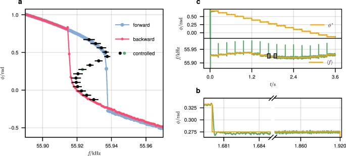
a Phase response curve of a frequency sweep with disabled control in forward (blue dotted line) and backward (red dotted line) direction. With enabled control, the unstable branch is tracked (black-filled circles). Control parameters are: KP = 12.6 kHz rad−1 and KI = 113 kHz rad−1 s−1. Error bars represent the mean standard deviation (see Methods section). b Transient behavior (green) of phase ϕ (top) and frequency f (bottom). The target phase ϕ⋆ (top) and the mean value of the last 2000 frequency values (bottom) are shown for comparison (orange). c Is a magnified view of the eighth control step indicated by rectangles in (b) and by a green-filled circle in (a).
a Phase ϕ(f, s) and b amplitude A(f, s) of an oscillating cantilever in attractive interaction with the silicon surface. The indicated mean tip-sample separation s corresponds to the amplitude setpoint (hard-surface approximation), which is varied in steps of 1.85 nm. An interactive version of these plots can be found in the Figshare repository.
Transient data for phase and frequency is shown in Fig. 4b, illustrating the dynamic behavior of the control scheme, particularly for the unstable branch. A magnified view of the transient phase evolution for one of the control steps is displayed in Fig. 4c. The target phase is approached quickly after each control step, while the remaining deviation is reduced on a slower timescale (see Fig. 4c), reflecting the typical behavior of the utilized proportional-integral (PI) control scheme, see equations (1) and (2). Finally, the phase clearly converges towards the target.
All control steps, including those on the unstable branch, reach the control target within the given period of time, where some minor oscillations are sufficiently damped by the control (see Fig. 4c). Occasional oscillations in the s-dependent curves visible in the frequency transients (Fig. 5, transients not shown) still result in much smaller uncertainties compared to the interpoint distance between two adjacent control steps.
Numerical simulations
In order to ensure the feasibility of our control approach prior to actual experiments, we employed a simple driven point mass model in common tip-sample interaction potentials, such as the Lennard-Jones or Derjaguin-Muller-Toporov model. However, quantitative a-priori modeling of unstable branches is essentially obstructed because the nature of the tip-sample system strongly depends on tip and sample materials, ambient conditions (particularly humidity), and time scales involved. Commonly accepted ingredients for a mathematical SFM model are a weak, long-range attractive interaction dominated by van-der-Waals forces (range of the order of 100 nm) and a short-range repulsive force caused by the Pauli principle (range of the order of 1 nm) and/or contact mechanical forces, e.g. treated within the Hertz model. Other attractive, repulsive, and dissipative contributions to the interaction force have been considered19,47,48, but crucial parameters (e.g., the dissipation coefficient) are essentially unknown. Hence, we did not try to find a physically accurate model but rather adhered to the simple Lennard-Jones model and chose parameters that qualitatively reproduce the experimental curves (Fig. 4).
Figure 6 shows simulation results for a Lennard-Jones potential with viscous dissipation as described in ref. 49. The control law (1) and (2), as well as the Least-Mean-Square (LMS) algorithm to obtain the Fourier coefficients on the fly, are realized with a similar time discretisation as in the experiment, while the equations of motion of the point mass oscillator are numerically integrated with a Runge-Kutta solver using adaptive step sizes. Despite the model’s simplicity, interaction forces and amplitudes are comparable to the experiment (see “Methods” section). Indeed the unstable branch is successfully tracked with suitable control parameters (KP = 0.4 ⋅ f0, ({K}_{{{{rm{I}}}}}=0.004frac{{f}_{0}}{{mbox{s}},}), f0 = 55 kHz), which are kept constant. The transient behavior in Fig. 6b shows that after some initial oscillations, the target phase and the instantaneous frequency are stable after a few ms, and thus confirms fast convergence to the stationary points in Fourier space. This proves that the feedback control scheme is indeed capable of stabilizing unstable states in the desired region of the bifurcation diagram.
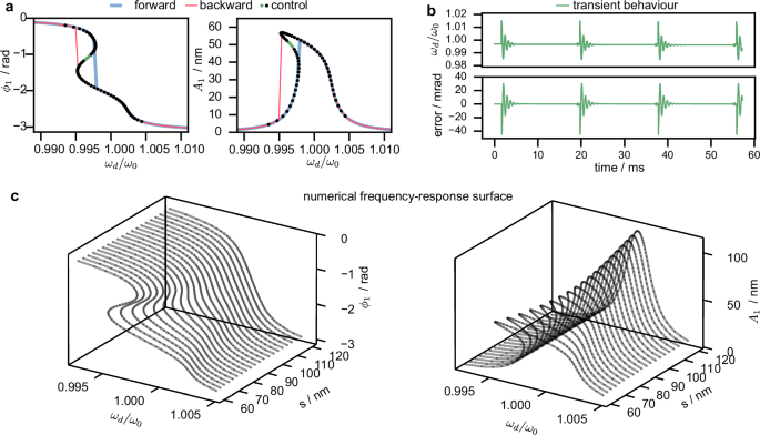
a Simulated frequency-response curves of a driven point mass in a Lennard-Jones potential with viscous damping at a separation of 60 nm. Black dots represent responses with enabled control, whereas red and blue lines correspond to backward and forward frequency sweeps with disabled control accordingly, indicating jump behavior at saddle-node bifurcation points. b Transient behavior of the driving frequency and phase-lag error towards formerly unstable periodic orbits, highlighted as green dots in (a). c Numerical frequency-response surfaces of phase ϕ (left) and amplitude A (right) where we choose the separation as the second bifurcation parameter.
Figure 6c shows the 3D two-parameter bifurcation diagram of the numerical model, i.e., frequency responses with enabled control for various tip-sample separations using the same control parameters for the entire simulation. All essential features, such as the initial shift of the frequency-response curve for large s, the occurrence of the unstable branch, its increasing length in the (ϕ, f) parameter space, and the emergence of a two-dimensional hidden fold are reproduced. This confirms the validity of experimental results, particularly the shape of the unstable branches. The remaining quantitative deviations are most likely due to the oversimplified model (interaction forces, point approximation).
Control behavior
While our results imply that tracking of unstable branches is successful, some uncertainties remain, resulting in potentially imprecise determination of the native states in the (f, s, ϕ)-phase space. Possible sources of errors are imperfect achievement of the control goal due to small oscillations around it, incomplete convergence, electronic noise resulting in fluctuations of the retrieved oscillation state (i.e., phase and amplitude), and variations of external forces, dynamically changing the characteristics of the oscillator. The main compromise we have to achieve is the total period of time available for the control sweep because thermal drift results in a time-dependent variation of the tip-surface distance and, hence, of the interaction force. Even sub-nanometer changes within a few minutes result in altered frequency-response curves, which impedes unambiguous characterization of the reference frequency sweeps (blue and red curves in Fig. 4a. In addition, a true stationary point in Fourier space does not exist, because the orbits lose their strict periodicity, and the phase to be targeted becomes a function of time. To avoid these complications, we limit the period of time per control step and rather occasionally accept a certain amount of remaining deviation from the control target. This may introduce a systematic error which, in principle, can be avoided by a more stable setup (e.g. employing active temperature control), by faster control schemes (e.g., beyond a simple PI controller), and by a more sophisticated termination criterion for each control step, hence saving some time, particularly in the less critical stable regions of the bifurcation diagram. Results shown in Figs. 4 and 5 are not affected by long-term drift, as evidenced by the coinciding (uncontrolled) frequency sweeps before and after the control sweep, respectively.
In our simple control approach, we selected static control parameters KP and KI, which apparently are not optimal for the entire range of the unstable branch. Although we obviously stay within the basin of attraction, we expect an even more robust behavior and faster convergence by a refined choice of parameters, e.g., in an adaptive manner50. The employed control not only enables stabilization of unstable branches, but also offers accelerated convergence to the stable states, resulting in much faster frequency sweeps. The effect is similar to that of decreasing the Q-factor via feedback, also known as Q-control22,51, which can drastically reduce the system’s response time to a changing excitation frequency.
Envisioned applications
Once successful stabilization on an unstable branch is achieved, the question of potential benefits emerges. We propose, that imaging on an unstable state—in the following referred to as unstable branch scanning force microscopy (UB-SFM)—potentially results in highly sensitive, yet robust imaging conditions, as argued in the following: consider the conditions for “soft” SFM, where the interaction between tip and sample is to be minimized, sometimes referred to as non-contact mode. A widely used strategy for achieving this goal is to increase the spring constant and decrease the oscillation amplitude, which has been particularly successful for the case of tuning-fork-based SFM operated in vacuum52, but is also pursued for cantilever-based microscopes in air.
A limiting factor, especially at ambient or liquid conditions, is the signal-to-noise ratio which ultimately sets a lower bound to the employed amplitude for practical purposes: using the amplitude modulation (AM)-detection scheme and typical cantilevers with normal spring constants k around 1 Nm−1 the noise level in the vertical z coordinate corresponds to about 0.1 nm34,38,53. Furthermore, amplitudes smaller than the sample corrugation result in a high probability of tip or sample modification, because of the predominant sideways forces exerted in such situations. Hence, for robust, long-term, and large-scale imaging, larger amplitudes are generally beneficial. This, however, is not easily possible in the attractive region of the tip-sample interaction because of the small range of amplitude setpoints required for this scenario, and due to the emergence of bifurcations (see Fig. 1), frequently encountered as erratic jumps of phase and amplitude in practical SFM experiments. Choosing the repulsive regime (often referred to as tapping mode), in turn, impedes the requirement of minimized tip-sample interaction. Forcing the system to remain on the upper stable branch in the attractive regime43 implies a weak amplitude dependence as a function of frequency due to the flat shape of the shark fin, hence, the sensitivity on tip-surface interaction forces is limited. Only on the unstable branch, large amplitudes can be combined with a high sensitivity (i.e., large (| frac{partial A}{partial f}|)) while entirely remaining in the attractive regime. Particularly when combined with the increasingly popular light-driven excitation scheme (e.g., via photothermal actuation)54, we expect UB-SFM to enable ultra-soft imaging conditions, being beneficial for soft samples, such as those encountered in biological systems.
Another application is touchless sensing of the effective tip-sample potential and dissipation at nanometric resolution. Further refinements of the interaction model, such as those collected in ref. 48 may result in quantitative data obtained simultaneously with imaging. As a side effect, erratic jumps between different stable orbits are avoided with enabled control, although other, dedicated approaches for this purpose have been proposed43. In a wider scope, our methodology is applicable to any micro- or nanomechanical system comprising a mechanical nanojunction, i.e., nearby interfaces with controlled (semi-) contact. Avoidance of stiction in controlled micro- or nanomechanical structures thus appears feasible, with numerous applications from sensors to miniaturized mechanical transmissions employing articulating surfaces.
An interesting topic for future investigation is also the question of how noise-reduction capabilities of a suitable control scheme, as shown for example in ref. 31, can lead to enhanced performance in an actual SFM experiment.
All these applications require implementing continuous scanning while stabilizing the unstable state. While this may be a technical challenge, based on our work, there are no fundamental obstacles.
Methods
Experimental realization
The experiment is based on a commercial SFM setup (NT-MDT NTEGRA Spectra Solar) with an external signal access module (see Fig. 3 for a simplified scheme). For versatile implementation of arbitrary control algorithms, signal generation and processing are accomplished by a real-time signal processing unit (RTSPU, ADwin Pro II, Jäger Messtechnik GmbH, Germany) based on a hybrid hardware combining a fast central processing unit (CPU), field-programmable gate arrays (FPGA), and fast 16-bit digital to analog and analog to digital converters (DAC, ADC). Time-discrete versions of equations (1) and (2) are used using a simple forward Euler method with a step-size of 1.2 μs, implemented within the ADwinC software package (Jäger Messtechnik GmbH, Germany). One of the RTSPU outputs is used for the actuation voltage applied to the dither piezo of the SFM, and the resulting cantilever deflection is measured by the integrated position-sensitive photodiode (PSPD) and fed to an RTSPU input for further processing. A second RTSPU output is connected to a high-voltage amplifier (Nanonis HVA4, SPECS Surface Nano Analysis GmbH, Germany), providing the z-piezo voltage for controlling the tip-sample separation.
Cantilevers with a low resonance frequency of nominally f0 = 45 kHz and high Q-factor (Q ≈ 400) are chosen (Extra Tall PointProbePlus SFM Tips, NanoWorld AG, Switzerland) for moderate controller speed requirements. Typical free oscillation amplitudes are ≈ 70 nm, and tip-sample distances are chosen such that the predominant forces remain attractive (with the exception of the respective lowest curve in Fig. 2a, b, where the repulsive force sets in as evident from the additional bifurcation point for each sweep direction).
All measurements are conducted on a Si(111) sample with a native oxide layer. Ambient humidity ranges from 17% to 36%. To minimize thermal drift and electromagnetic noise, the SFM setup is enclosed by a grounded protective box. The tip-sample separation is estimated from the oscillation amplitude, calibrated by force-distance curves on the Si sample. The phase is used as the control target because compared to the amplitude, it is more distinct between the two stable states (see Fig. 2), and it behaves monotonically within the region of the unstable branch, simplifying the sampling algorithm. Each experimental control run consists of frequency sweeps (forward/backward) with disabled control, followed by the controlled phase sweep from high to low values, and another set of frequency sweeps (forward/backward). The uncontrolled frequency sweeps serve as a reference and enable identification of the approximate location of the unstable branch in the (f, ϕ) plane. We used control gains in a range from KI = 113 kHz rad−1 s−1 to 202 kHz rad−1 s−1 and KP = 11.4 kHz rad−1 to 12.6 kHz rad−1. Typical durations are ≈ 1.2 μs per individual control cycle, resulting in about 240 ms for one control run (i.e., for each value of the target phase ϕ⋆). This reflects a compromise between minimal drift and good data quality. The last ≈ 40% of data points of each control step are used for deducing statistical figures (i.e., mean and its standard deviation), represented by data points and error bars plotted in Fig. 4a (where the phase error is much lower than the size of the graph markers, hence hardly visible). A full version of the ADwinC code, including nLMS implementation, signal generation, and control algorithm, can be found in the Figshare repository.
For the response surfaces A(f, s) and ϕ(f, s) as shown in Fig. 5 the tip-sample separation is varied in steps of 1.85 nm between each control run. This is done by setting the respective new z-piezo voltage and employing a PI feedback loop to stabilize the z position (i.e., keeping the amplitude constant). Then, the feedback is disabled again, and the next control run is started. Due to technical restrictions on the communication between the RTSPU system and the personal computer, only part of all control runs is available as a full data set for the response surface. For control steps without full datasets, only the final values of phase and frequency are taken as a result, hence these data points show increased scatter.
Phase extraction
For both, experiment and simulation, fast phase extraction is crucial. Our approach is based on a least-mean square algorithm. In dynamic mode SFM, a mono-harmonic excitation force of the form (Gamma sin (psi (t))) is applied. We observe the deflection response x(t) using a truncated Fourier series
We will refer to
as the harmonic state, to the Fourier coefficients X0, Xi,s, Xi,c as the harmonic variables, which change at a slow timescale (Tgg 2pi /min {omega }_{i}), and towards N as the truncation order. To obtain the harmonic variables, which coincide with the Fourier coefficients, we use a Least-Mean-Square (LMS) algorithm in contrast to the standard Lock-In-Amplifier setup. For general decomposition practices the LMS algorithm was introduced for noise canceling applications in45, in atomic force microscopy this method was investigated in46, for continuation purposes the LMS algorithm was first used in55, a comprehensive overview of general adaptive filters can be found in56. Time-explicit update equations for the harmonic state X can be found in the “Methods” section.
In the experiment as well as in the simulation, we get information on the current tip displacement x with a sampling time Δt. Using the index as the time discretisation x(nΔt) = x∣n, the LMS Algorithm updates the harmonic state X time explicitly by
where μ denotes the step-size. We exploit the linear parametric form of the truncated Fourier series and
describes the current basis vector with the instantaneous phase ψ∣n of the actuator (Gamma cos psi {| }_{n}) as an argument to ensure synchronized clocks between measurement and forcing. The error e∣n is the difference between current measurement x∣n and approximation of the displacement (widetilde{x}{| }_{n}={X}^{top }{| }_{n}c(psi {| }_{n})). In quadrature interpretation we obtain amplitudes Ai and phaselags ϕi from harmonic state X via
Whereas in experimental settings we only use the fundamental i = 1 to manipulate the driving frequency, in principle we can take into account higher harmonics. Experimental data of the deflection signal (see Supplementary Fig. 1) illustrates that mono-harmonic approximation of the measured signal is reasonable.
Simulations
For simulations, we use a normalized time, which can be seen as the number of cycles at the natural frequency ω0 of the cantilever. In the following, we will refer to t as the normalized time. The driven point mass in the Lennard-Jones potential with viscous damping can then be written as a coupled ordinary differential equation (ODE)
and is integrated numerically in Julia by an adaptive Runge-Kutta solver TSIT5() of DifferentialEquations.jl57. We thereby choose the parameters, k = 0.7 Nm−1, Q = 400, s = 60 nm, σ = 2.8 nm, f = 130 nm, ω0 = 2π ⋅ 55000 rad s−1, V0 = 4.2 ⋅ 10−18 J, γ = 0.6 ⋅ 10−31. In the open loop and also closed-loop simulation we vary the normalized driving frequency (frac{{omega }_{{{{rm{d}}}}}}{{omega }_{0}}) after the transients die out by a discrete callback. In order to check convergence towards a steady state we use an adapted Welford algorithm in combination with a circular buffer. The variance Σ, and mean value 〈y〉 of the circular buffer with head H can be obtained time explicitly by
In our case, we store transient phase-lag values ϕ1 in a circular buffer of length L = 40 with a sampling frequency of 15.3 cycles at the resonance frequency. We identify steady-state behavior and do a continuation step in the phase-lag target ({phi }_{1}^{star }) once the conditions
are fulfilled. Hereby we choose (Delta {phi }_{1}^{star }=0.0005) rad and σtol = 0.00001 rad. For the LMS algorithm, we truncate the Fourier series at the 4th harmonic, use the step-size μ = 0.01, and update the harmonic state as well as the instantaneous phase ψ, 10 times every cycle at the natural frequency ω0, which corresponds to Δt = 0.01. For further details and exact implementations we would like to refer to the code, which is available in the public GitHub repository.
Responses