FALCON: Fourier Adaptive Learning and Control for Disturbance Rejection Under Extreme Turbulence

Introduction
Turbulent atmospheric winds often contain transient flow disturbances and aerodynamic forces that can affect a variety of systems and structures1. These forces are particularly significant for aerodynamic technologies like unmanned aerial vehicles (UAVs) and wind turbines, which rely on fluid interaction for regular operation and can be damaged when operating in turbulent conditions2,3,4. Developing active control strategies to mitigate the effects of these turbulent forces is one of the most important challenges in the safe deployment of UAV technologies or extending the lifetime and reliability of wind turbines5,6,7. Developing and utilizing complex flow models for control is challenging in real-time due to sensor noise, low-latency, and high-frequency control requirements8,9,10. For example, modeling the flow requires advanced computational fluid dynamics (CFD) solvers that are often too slow for real-time application and fail under noisy settings11.
Conventional control strategies for UAVs, such as proportional-integral-derivative (PID) controllers, are designed to reactively correct inertial deviations from the desired trajectory without taking into consideration the underlying flow dynamics or the source of the disturbance12,13,14. These approaches are often insufficient for maintaining stability in extreme atmospheric turbulence, which prevents deployment of these technologies in safety-critical scenarios such as deploying unmanned aerial vehicles (UAV) in densely populated urban areas15,16,17, such as Fig. 1A. A line of work proposes adding Dryden or von Karman turbulence models, a simplified side dynamics, as a correction to the base dynamical model18,19,20. Such corrections are inspired by first-order physics and introduce ordinary differential equations (ODE) correction to the UAV dynamics. These approaches are also often used in practice and come with the limitations that the correction is known, and an Euler method with fine time resolution is needed for the ODE correction.

A Complex airflow structures in urban environments. B The wing has 9 sensors to measure the airflow (8 equally spaced pressure taps and 1 pitot tube) and is mounted on a one-dimensional load cell to measure the lift. Trailing-edge flaps change orientation to manipulate the aerodynamic forces. C Experiment setup to create irregular turbulent wake of a bluff body under high wind speeds. D Smoke visualization of the turbulent wake of a cylinder at a smaller Reynolds number. This image is obtained at the Caltech Real Weather Wind Tunnel system at a significantly lower flow speed than the experiments conducted in this work for visualization purposes. The actual flow conditions used in our studies were too turbulent to have clear smoke visualization. E Under a uniform flow U∞, symmetric airfoils do not have any vertical aerodynamic forces on them when they are aligned with the airflow. However, altering the position of a trailing edge flap on the airfoil can modify the lift coefficient CL, yielding an upward or downward aerodynamic lift force. F Outline of FALCON, a model-based reinforcement learning framework that allows effective modeling and control of the aerodynamic forces due to turbulent flow dynamics and achieves state-of-the-art disturbance rejection performance.
In contrast, biological swimmers and flyers have the ability to directly observe and respond to the physics responsible for changes in motion21,22,23,24. By drawing inspiration from these biological systems, there have been considerable efforts to improve control strategies for UAVs by using easily measurable flow quantities, such as pressure, to anticipate and mitigate the effects of turbulent disturbances25,26,27,28,29,30. The majority of these works again utilize the flow-sensing information within PID control frameworks which limits their desirable performance to low velocities25,26,27,28 or they consider uniform wind/flow scenarios where the eddies and gusts have smaller scale than the UAVs which result in small aerodynamic disturbances29,30.
To tap the potential of flow-sensing in designing disturbance rejection policies, reinforcement learning (RL), a machine learning area, has been recognized as a promising framework, due to its ability to learn and adapt to the unmodeled dynamics and design nonlinear policies with various objectives. Most of the prior works on RL for flow control have focused on model-free RL techniques and developed in CFD simulations. Model-free RL methods do not construct an explicit model of the system dynamics and aim to learn the control policies directly through interactions with the system31. Therefore, they are the most intuitive choices for policy design in environments difficult to model such as turbulent flow dynamics. Among these model-free RL works, Bieker et al.32 introduced a novel framework with online learning to predict and control flow in a 2D CFD simulation. Gunnarson et al.33 introduced an algorithm to navigate a simulated “swimmer” across an unsteady flow in a 2D simulation. In the experimental studies, Fan et al.34 demonstrated the first experimental applications of model-free RL in fluid mechanics. Recently, Renn and Gharib35 used a model-free RL method for controlling the aerodynamic forces on an airfoil under turbulent flow in an experimental setting (similar to the one considered in this work) and achieved state-of-the-art disturbance rejection performance, outperforming PID control. They also documented that the power spectrum of the turbulent flow at high Reynolds numbers is dominated by the low-frequency components which inspired the development of the algorithm in this work. However, despite this strong empirical performance, their method suffers from well-known limitations of the model-free RL methods, namely, extensive and laborious data collection, and brittle policies.
In this work, we take on the challenge of designing a model-based RL framework for flow-informed aerodynamic control in a highly turbulent and vortical environment to overcome these limitations. Unlike their model-free counterparts, model-based RL methods pursue joint objectives of model learning and policy optimization36. They are strong alternatives to model-free methods due to their sample efficiency, ability to adapt to changing conditions and to generalize to unseen conditions via the learned model. Moreover, most real-world systems are governed by physics, which can be incorporated into model learning. This also enables them to generalize better to out-of-distribution samples, which is crucial in safety-critical tasks. However, despite these promises, most of the current model-based RL methods are rarely implemented in real-world systems due to their need for highly accurate models and the challenges that partial observability brings.
In most real-world dynamical systems, the system state is hidden, and instead, the controlling agent observes a nonlinear and noisy measurement of the state, e.g. through sensors. This partial observability brings uncertainties in modeling the system dynamics and designing the policies37. It also violates the common design assumption of the Markov property in the collected samples, which significantly complicates the modeling task38. These challenges make model-based RL remarkably difficult in real-world systems. To remedy these challenges, the majority of the model-based RL methods rely on the expressive power of deep neural networks (DNN) in modeling the dynamics. However, these approaches require a vast number of samples and usually yield black-box models. Thus, these methods are most relevant in stationary and safe environments such as robotic manipulations39. However, under unsteady conditions such as complex turbulent flow fields, we require efficient and adaptive modeling for generalizable learning.
In this article, we propose an efficient model-based RL algorithm, Fourier Adaptive Learning and Control (FALCON), for online control of unknown partially observable nonlinear dynamical systems, in particular for disturbance rejection under extreme flow conditions for which the turbulence dynamics and future events are a priori unknown (Fig. 1F). FALCON leverages the domain knowledge that the underlying turbulent flow dynamics are well-modeled in the frequency domain and that most of the energy in the turbulent flows is present in low-frequency components35,40. Therefore, it learns the underlying partially observable system in a succinct Fourier Series basis. In short, FALCON constructs a highly selective and nonlinear feature representation of the system in which the dynamical evolution is approximately linear (in the feature space), resulting in an end-to-end highly nonlinear and accurate model of the underlying system dynamics. The Fourier coefficients provide good inductive bias to learn this cross-coupling automatically from observations. The soundness of model learning using constructed Fourier bases is theoretically guaranteed, and the algorithm design in this work is mainly towards low error in the next step prediction. In this work, we evaluate the accuracy and soundness of the learned model using controller performance equipped with the learned model, which is the quantity of interest in RL and control. The low error prediction error is sufficient to achieve the learning and control guarantee and arrive at the proposed practical algorithm. FALCON consists of two main parts: a warm-up phase and adaptive control in epochs phase. In the warm-up phase, using only a small amount of flow data (35 seconds-equivalent to approximately 85 vortex shedding interactions) FALCON recovers a succinct Fourier basis that explains the collected data and enforces that this learned basis is mostly composed of low-frequency components following the prior observations on turbulent flow dynamics. It then uses this basis to learn the unknown linear coefficients that best fit the acquired data on the learned Fourier basis during the adaptive control phase.
In the control design, FALCON uses model predictive control (MPC) and efficiently solves a short-horizon planning problem at every time step with the learned system dynamics. This recurrent short-horizon planning approach allows FALCON to adapt to the sudden changes in the flow while designing more sophisticated policies that consider future flow effects in contrast to the conventional purely reactive controllers. Moreover, the simple yet physically accurate dynamics learning approach of FALCON further facilitates the effective control design, which results in a sample-efficient and high-frequency control policy. During the adaptive control phase, FALCON refines its model estimate, i.e., the linear coefficients, in epochs in order to improve the learned model, which in turn improves the performance of the MPC policy. Overall, FALCON provides a simple, efficient, and interpretable dynamics modeling and an adaptive policy design method for the flow-predictive aerodynamic control problem and significantly outperforms the state-of-the-art model-free RL methods and conventional control strategies, i.e., PID, using only a total of 9 min of training data representative of approximately 1300 vortex shedding cycles. FALCON easily incorporates the physical and safety constraints in the policy design and builds on a fundamental understanding of how well nonlinear systems can be approximated and how these approximation errors affect the control performance, which we support with rigorous theory.
We implement FALCON on an experimental aerodynamic testbed that abstracts the fundamental physics involved in flight through a turbulent atmospheric flow and is specifically relevant for fixed-wing UAV applications. This testbed consists of a 3D-printed airfoil with actuated trailing edge flaps and an array of pressure sensors to measure the surrounding flow (Fig. 1B). The system is mounted in a closed-loop wind tunnel on a load cell measuring the aerodynamic lifting force acting on the airfoil. The testbed is placed in the wake of a bluff body at a Reynolds number of 230, 000, which generates a highly turbulent and vortical environment (Fig. 1C). This setting is on the upper-intermediate range of turbulent spectrum, and follows the description of realistic fixed-wing UAV flights with indicated Reynolds numbers ranging from 30, 000 to 500, 00041. The aerodynamic control goal is set to minimize the standard deviation of the lift forces by adjusting the position of the trailing-edge flaps in response to incoming disturbances with the help of flow sensors (Fig. 1E). In free flight, this would be equivalent to minimizing the inertial deviations along the lifting axis.
Through these wind tunnel experiments, we report that FALCON achieves 37% better disturbance rejection performance than the state-of-the-art model-free RL method35, using only a single trajectory and 8 times less data. Moreover, we document a performance improvement of 45% over the conventional reactive PID controller. Overall, we find that the superior performance of FALCON is consistent over independent runs in the highly irregular unsteady turbulent flow dynamics, demonstrating the adaptation and generalization capability of FALCON to the unseen conditions.
Results
Novel Model-based RL Framework: Fourier Adaptive Learning and Control (FALCON)
FALCON has two main phases: a warm-up and an adaptive control in epochs phase (Fig. 2). The warm-up phase is a short initial period, where FALCON collects initial data about the fully unknown system. The goal is to purely explore the system and recover a coarse model of the dynamics. To that end, FALCON executes smooth and safe actions, i.e., time-correlated Gaussian inputs, that safely excite the system (see Methods for other variants). Since FALCON relies on pressure sensors on the airfoil to measure the system dynamics, it operates under partial observability. The chaotic dynamics of the systems undergo quick transients from their earlier states, forgetting them, making the current dynamics more heavily dictated by recent observations and actions than earlier ones. To overcome the uncertainties that partial observability brings, FALCON uses the recent history of actions and measurements to model the system dynamics. At the end of the warm-up phase, FALCON uses the data collected to learn the most relevant Fourier basis that explains the observed turbulent dynamics. FALCON is data efficient and requires only 35 s of flow data during the warm-up phase to recover an informative Fourier basis. This 35 s of flow data include fewer than 1500 samples taken over a period spanning approximately 85 vortex shedding events.
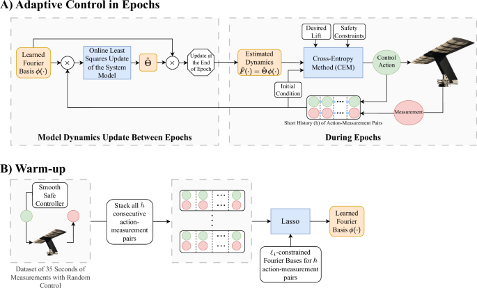
It consists of two phases: Warm-Up and Adaptive Control in Epochs. A Adaptive Control in Epochs: FALCON models the system dynamics as a linear map of the representation of a short history (h-length) of action-measurement pairs in the succinct Fourier basis learned in the warm-up phase. FALCON learns the unknown linear coefficients that best model the dynamics via online least squares. It updates the estimated system dynamics, i.e., the linear coefficients, at the end of each epoch, and during the epochs, it uses Cross-Entropy Method (CEM), a sampling-based MPC method, to control the airfoil under extreme turbulence using the estimated system dynamics while satisfying desired lift and safety requirements. B Warm-up: It is a one-time 35 s process before starting the adaptive control phase for safely collecting some exploratory data about the unknown system to recover a relevant Fourier basis to be used in learning and adaptive control. To achieve this FALCON forms h-length subsequences of action-measurement pairs (a short history) from the safely collected dataset and solves the lasso problem on the ℓ1-constrained Fourier basis representation of these subsequences. FALCON selects the Fourier basis vectors that correspond to non-zero coefficients in the solution of the lasso problem as the succinct Fourier basis ϕ(⋅) for the entire adaptive control in epochs phase for learning and control of the system.
FALCON incorporates several key features that achieve data and computational efficiency in the basis learning process. In particular, FALCON uses ℓ1-constrained (sparse) Fourier basis, as well as least absolute shrinkage and selection operator (lasso)42 to recover a succinct basis representation (see details in Methods). This improved basis selection yields a significantly compact model representation while allowing physically accurate modeling of the underlying system dynamics due to the low-frequency dominant choice of Fourier basis, i.e., sparse Fourier basis vectors43. Indeed, spectral methods and modal analyses for modeling turbulent fluid dynamics are well-established concepts44,45, and it is known that large eddies with low frequencies contain the most energy in turbulent flows40. This inductive bias in modeling via sparse Fourier basis reduces the number of samples required to learn the turbulent dynamics with small modeling errors and alleviates the computational burden in the predictive control design, facilitating high-frequency control actions. FALCON allows flexibility in the basis learning procedure such that the number of Fourier basis used in model learning could be easily adjusted based on the prior knowledge of the system dynamics, the difficulty of the learning task, and the computational budget.
After recovering a succinct Fourier basis for model learning, FALCON starts the adaptive control in epochs phase, Fig. 2A. It estimates the model dynamics as a linear model in the learned Fourier basis and aims to learn the unknown linear coefficients that best fit the acquired data onto this basis. In particular, FALCON solves an online least-squares problem that has a closed-form solution to learn these linear coefficients. This interpretable and lightweight model learning allows online and/or batch updates for computational efficiency and comes with strong learning theoretical guarantees for the robustness of modeling (see Materials).
During this phase, FALCON designs an online control policy based on this learned model while improving the system dynamics model in an online fashion over time. This process goes in epochs with doubling duration, i.e., each epoch is double the length in seconds of the previous epoch, where at the end of each epoch FALCON updates its linear coefficient estimates on the model for better-refined dynamics modeling and control. This epoch schedule reduces the number of model updates towards the later stages of adaptive control where the dynamics are already well-modeled and only small tuning is required to further improve. We would like to highlight that FALCON is a single trajectory algorithm in the sense that it does not require a reset between epochs, which makes it efficient in the data collection process.
As the online control policy, FALCON uses model predictive control (MPC) with the estimated model dynamics to design the control inputs during the adaptive control phase. For controlling nonlinear dynamical systems such as aerodynamic control in turbulent flow considered in this work, finding the optimal solution to the control problem is usually challenging46. As a practical and efficient alternative, MPC policies have been the dominant choice for designing controllers in nonlinear dynamical systems47. Given the initial conditions, the transition dynamics (can be an estimated model or a nominal model), the running costs, and the terminal costs at any given time step, the objective in MPC is to solve a short horizon optimal control problem and execute the first action of the solution sequence. This process is then continued as we gather new observations. Intuitively, instead of trying to solve the challenging global optimal control problem, MPC myopically solves a locally optimal control problem. Usually physical or safety constraints on actions, observations, and dynamics are added in the MPC formulation due to its simplicity of implementation. The choice of the MPC policy depends on the control task. In general, the MPC policies are either optimization-based48 or sampling-based49. However, sampling-based methods are usually preferred in model-based RL due to challenging nonlinear system dynamics and complicated cost and constraint functions50.
Therefore, at every time step of the adaptive control phase, FALCON deploys a Cross-Entropy Method (CEM) policy, a sampling-based MPC policy49, to design control actions using the most recent system dynamics estimate as the transition dynamics. CEM maintains a distribution, predominantly Gaussian, to sample action roll-outs for the short planning horizon and iteratively updates this distribution to assign a higher probability near lower cost action sequences based on the estimated system dynamics. After a certain number of updates, it executes the first action on the lowest cost-achieving action sequence in the sampled roll-outs (see further details of MPC design and CEM in particular in Methods). FALCON takes in the most recent short history of actions and measurements as the initial condition for short-horizon MPC objective. For the running and terminal control costs FALCON can utilize any kind of cost functions as long as they can be evaluated efficiently depending on the control task. In our experiments, we design the cost function of FALCON based on our aerodynamic control objective such that FALCON avoids large lift forces and prevents rapid changes in lift forces and fast/jittery action changes. The first two design choices are clear from the control goal, i.e., minimizing the mean and the standard deviation of the overall lift forces, whereas, the last one is more subtle. In our experiments, we observed that non-smooth changes in actions cause additional lift forces on the airfoil (see further discussion on cost design choice in Materials). Furthermore, in the policy design FALCON includes action constraints due to mechanical restraints of the aerodynamics testbed as we shortly discuss in the next section.
FALCON can easily include further safety or physical constraints within its MPC framework. This makes FALCON a reliable algorithm for safety-critical tasks such as free flight through turbulence. Moreover, the recurrent short-horizon planning approach through CEM allows FALCON to design sophisticated policies that consider future flow effects through the use of estimated model dynamics. Thus, rather than designing purely reactive policies that cancel out the instantaneous aerodynamic forces, FALCON designs flow-predictive disturbance rejection policies which aim to minimize the lift forces while accounting for unsteady flow dynamics. In this way, FALCON adapts to sudden changes in the flow while avoiding overcompensation of the aerodynamic disturbances by maintaining an overall understanding of the flow field. The simple, yet physically sound and accurate dynamics learning approach of FALCON facilitates this effective control design, which results in a sample-efficient and high-frequency (42 Hz) state-of-the-art control policy with generalizable performance.
The construction of FALCON is modular such that different basis functions, e.g. wavelets51, could be utilized in learning the underlying system dynamics depending on the domain knowledge about the system, while the MPC framework could be selected based on the specific needs, e.g. optimization-based MPC for simpler model dynamics. This interchangeable design of FALCON makes it a viable model-based RL method for designing diverse online/adaptive control strategies for various tasks (see Discussion). Moreover, it also allows for the derivation of strong theoretical guarantees for the robustness of model learning and the control performance under modeling error, see the Methods section. In particular, we prove that a wide range of partially observable nonlinear dynamical systems such as dynamical systems governed by partial differential equations could be learned with arbitrary modeling error using Fourier basis for FALCON. We also show that this effective model learning allows stable control design for robust MPC frameworks and the systems controlled by FALCON follow a trajectory close to the systems regulated with the same MPC policy that has access to perfect system dynamics information. Finally, we formalize the performance guarantee of FALCON such that the control performance of FALCON converges to the idealized MPC controller that knows the perfect system dynamics. These rigorous theoretical results display the reliability of FALCON while attaining state-of-the-art performance in predictive flow control.
Experimental aerodynamic testbed
In this work, we abstract the problem of stabilizing an aerodynamic system under turbulence to basic components while maintaining the core complexity of the physics involved. We utilize an experimental aerodynamics testbed that captures and generalizes the fundamental physics involved in flight through a turbulent environment35. The aerodynamic testbed consists of a symmetric generic airfoil with motorized trailing-edge flaps and integrated flow sensors (Fig. 1B). The trailing-edge flaps have an actuation range of [-40∘, 40∘], and are mapped linearly from the action space of [−1, 1], yielding 1-dimensional control action per time step. Similar to flap systems on conventional airplanes, actuating the trailing-edge flaps generates a lifting force that can offset the aerodynamic forces associated with flow disturbances as shown in Fig. 1E. The testbed is equipped with nine sensors which are placed 10cm apart along the spanwise axis. Observations of the surrounding flow are measured through a series of eight pressure tap flow sensors built into the body of the airfoil, with a single pitot-static tube located at the center of the airfoil. The pressure taps, placed near the leading edge of the airfoil, provide valuable information on incoming pressure differentials between the upper and lower surface of the airfoil. The pitot-static tube measures the total pressure of the incoming flow which is approximately proportional to the mean velocity of the flow. The aerodynamic testbed is mounted on a one-dimensional load cell which is used to observe the lift forces acting on the airfoil, which serves the same effective role as an inertial measurement unit on conventional UAVs. Combined with nine flow sensors, we obtain 10-dimensional measurements per time step. Further details on aerodynamics testbed design are provided in Methods.
Turbulent environment
We study control in the context of a canonical problem in fluid dynamics: the turbulent wake of a bluff body. When placed incident to winds, bluff bodies produce an oscillating vortical wake commonly known as a Kármán vortex street52. At sufficient wind speeds, this wake becomes highly turbulent and can result in significant forces43, as visualized with smoke in Fig. 1D. This photo is captured at Caltech Center for Autonomous Systems and Technologies (CAST) fan-array wind tunnel with a standard cylinder at a lower wind speed than the experiments presented in this work. Figure 1D depicts the turbulent wake of the cylinder where the vortex shedding is irregular. This phenomenon is famously responsible for the 1940 collapse of the Tacoma Narrows Bridge53.
All of the quantitative results in this work were obtained from the experiments conducted in Caltech’s Lucas Adaptive Wall Wind Tunnel, a closed-loop wind tunnel. As discussed previously, our experiments were performed in the wake of a bluff body at a mean flow speed of 6.81 m/s, which corresponds to a Reynolds number of ReD = 230,000 over the bluff body. The bluff body consisted of a cylinder with a diameter of 30 cm with a normal flat plate fixed asymmetrically that increased the effective diameter to 53 cm, as shown in Fig. 1C. This construction is used to encourage vortex dislocation which results in less regular vortex shedding events54. Further, the bluff body was mounted to the walls of the tunnel with elastic cords to allow for dynamic oscillations which may also encourage less regularity in shedding events (see Methods for details).
We used particle image velocimetry (PIV) to visualize a portion of the turbulent flow field in our experimental environment (see Methods for details). Figure 3 presents the PIV measurements of the vorticity field contextualized in the wind tunnel. The complex vorticity patterns clearly demonstrate the chaotic and unsteady turbulent flow dynamics, with strong three-dimensional effects likely present in our experimental setting. Moreover, through hot-wire anemometer measurements in the wind tunnel, we record a turbulence intensity of 10.8%.
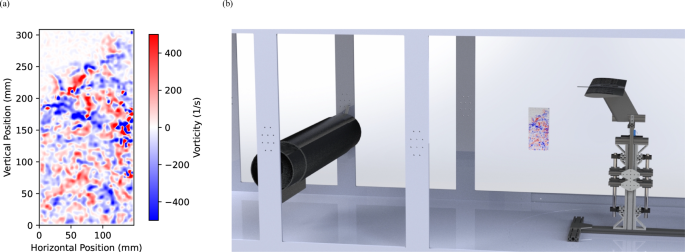
a Particle Image Velocimetry (PIV) Visualization of the Turbulent Flow Field. b Depiction of PIV measurement location in the wind tunnel
Baseline control methods
To test the performance of FALCON, we deploy several RL baselines and the industry-standard responsive control strategy of PID (Proportional-Integral-Derivative) control in our aerodynamics testbed. In particular, we compare FALCON with the twin delayed deep deterministic policy gradient algorithm TD355, its variant known as LSTM-TD356, and soft actor-critic algorithm SAC57 (see Methods for a detailed overview of these methods). These methods are the state-of-the-art off-the-shelf model-free RL methods deployed in many real-world control tasks34,35,58,59. They are off-policy actor-critic algorithms that utilize neural networks for control policies. Off-policy methods are usually preferred over on-policy methods in real-world dynamical systems with unsteady dynamics since they can learn from a wide range of experiences, including observations from previous policies, which makes them more robust to changes in the environment. Another advantage of off-policy methods is that they can learn an optimal policy even when the current policy is significantly sub-optimal, which is usually the case for challenging real-world control tasks due to the lack of clearly superior expert policy. These all combined allow off-policy methods to be more stable during the learning process, which leads to better convergence and generalization performance31.
The TD3 algorithm has previously demonstrated success in experimental flow control in different settings34. To improve performance in partially observable systems, such as the turbulent flow dynamics measured by sensors, LSTM-TD3 utilizes recurrent long-short-term memory (LSTM) cells in the neural network structure of TD3. The addition of LSTM cells has been previously shown to improve the performance in prediction and control of highly unsteady stochastic environments like turbulent flow fields60. In particular, recently, LSTM-TD3 has been demonstrated to achieve state-of-the-art performance in disturbance rejection in a similar experimental setting studied in this work35. Therefore, LSTM-TD3 provides the ultimate baseline for FALCON. In their implementations, both TD3 and LSTM-TD3 have nearly identical parameters besides the additional LSTM structure of LSTM-TD3 for an additional memory element in the policy. While TD3 and LSTM-TD3 provide deterministic policies, SAC designs stochastic policies, which is shown to achieve significant success in various real-world tasks such as quadrupedal robots and voltage control57,61. It provides a sample efficient alternative policy design method compared to TD3 and LSTM-TD3.
Due to the stochasticity in the process of training RL algorithms, we trained each of the agents presented here with three independent random seeds and present the average training results to display their performances. Unlike FALCON, the model-free methods work in episodes with reset for retraining. We train the model-free methods for 200 episodes of 800 samples per episode and use the best-performing agent for each algorithm in presenting their final performance. The feedback gains of the PID controller were tuned manually to achieve constant zero lift using the readings of load cell measurements. In our experiments, we run an exhaustive grid search over the feedback coefficients and report the best-performing controller. All methods, including FALCON, are implemented with 42 Hz sensing and control frequency.
Superior performance and sample efficiency of FALCON
First, we provide the results on the training of the methods. In presenting the training behavior, we exclude the warm-up of each method. Note that the warm-up phase of FALCON requires only 1500 samples, which corresponds to approximately 85 vortex shedding cycles from the upstream bluff body. Figure 4 shows the moving average of the mean and standard deviation of the lift forces on the airfoil for the best-performing policy of each method over the first 42,000 samples collected. In this plot, while the data collection procedure of FALCON does not pause in between model updates (epochs), the model-free algorithms pause (end of their episode) and train for some time to update their policy. From these plots, we observe that FALCON quickly finds the unknown linear coefficients to represent the system dynamics in the learned Fourier basis and achieves significantly better performance than model-free methods with fewer samples. We also note that during the 40,000 sample period shown, FALCON has only 25 learning updates while the other algorithms shown have 50. As the model-free algorithms used for comparison typically require more data, we trained these algorithms for a total of 200 episodes (equivalent to 160,000 samples), the remainder of which can be seen in Fig. 5. The training behavior of FALCON indicates that FALCON agents consistently improve throughout training and require significantly less training time to outperform state-of-the-art model-free methods due to its physically accurate model learning procedure and efficient control design.
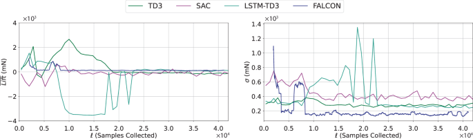
Evolution of the mean ((overline{,text{Lift},})) and standard deviation (σ) of the lift forces for the best-performing agents of each algorithm shown over the first 40,000 samples. The full training performance for the model-free algorithms can be found in Fig. 5.
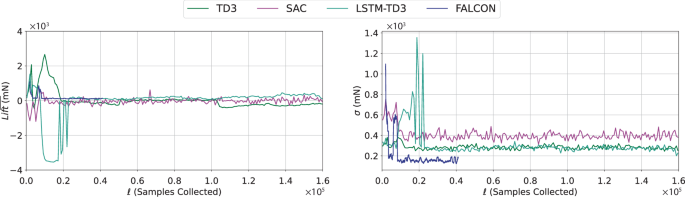
Evolution of the mean ((overline{,text{Lift},})) and standard deviation (σ) of the lift forces for the best-performing agents of each algorithm shown over the full 200 episodes for which the model-free algorithms were trained (160,000 samples).
Even though FALCON can suffer from model uncertainty and execute sub-optimal actions at the beginning of training due to unsteady flow dynamics (see the outlier bump in the standard deviation of lift in Fig. 4 around t = 6000), FALCON effectively explores the state-space to improve the accuracy of the model and hence the performance of the controller to bring the standard deviation in the lift forces to desirable values. After 10,000 samples, i.e., 4 min of training of FALCON, the average standard deviation of lift forces on the aerodynamics testbed remains stable at a level significantly better than other tested methods. Similarly, the mean lift forces achieved via FALCON consistently outperform that of model-free methods.
Among the model-free methods, Fig. 4 shows that LSTM-TD3 is the second best-performing algorithm by outperforming TD3 slightly, while SAC fails to achieve acceptable performance. Note that LSTM-TD3 and TD3 share the same policy constructions except the LSTM part that adopts latent states in the policy. Combined with the superior performance of FALCON, this highlights the importance of a latent state representation in achieving desirable learning and control performance in partially observable real-world settings. Similar to FALCON, LSTM-TD3 achieves consistent performance after sufficient samples, yet it requires an order of magnitude more than FALCON. Despite our significant efforts in hyperparameter tuning, SAC agents failed to learn desirable policies that minimize the aerodynamic forces. Even the best-performing agent significantly underperformed compared to other model-free policies, which indicates that stochastic policies such as SAC might not be suitable for controlling unsteady dynamical systems.
From our experiments, we observe that FALCON is more robust to hyperparameter tuning and has a notably more stable training process (Fig. 4) compared to model-free methods. In particular, in our training process, tuning FALCON requires only a few trials on the history of modeling (number of past observation-action pairs used), the sparsity weight in lasso for recovering a succinct basis, and the planning horizon for CEM. On the other hand, model-free methods require extensive hyperparameter search to achieve some learning behavior. This extensive search is significantly time-consuming and laborious in real-world problems, e.g. the training process of model-free methods corresponds to an hour of training for each hyperparameter configuration in our setting. This process becomes unfeasible in online resource-constrained settings, which are typically the scenarios for adaptive control systems.
Our experiments overall showed that FALCON consistently achieves better and more stable training performance than model-free methods while converging to its optimal policy with orders of magnitude fewer samples. This superior performance and sample efficiency show that the simple yet efficient partially observable dynamics modeling approach of FALCON reduces the complexity of the aerodynamic control under turbulence problem significantly. Combined with the efficient predictive control design, FALCON agents learn to reject the flow disturbance effectively. The model learned by FALCON also aligns well with established knowledge regarding spectral energy content; in particular, the improved basis selection with ℓ1-constraint and lasso enforces the model to have relatively low frequencies corresponding to the dominant energy-containing eddies. In our experiments, we observe that FALCON recovers model estimates which put significant weight on the low-frequency basis, e.g. DC components, and some high-frequency components (see Methods). This shows that via using the relevant basis for learning, FALCON learns a physically meaningful model, which contributes to training stability and disturbance rejection performance of FALCON.
To further investigate the effect of the concise Fourier basis-based model learning approach of FALCON, we implemented a reasonably sized deep neural network for model learning and combined it with CEM-based policy design as FALCON. However, despite our significant efforts in tuning, this approach failed to learn a reliable model for control design due to unsteady and chaotic flow conditions, which resulted in a performance significantly worse than the reported algorithms in this work. This outcome highlights that black-box dynamics modeling methods such as deep neural networks can fail in unsteady systems such as turbulent flow dynamics.
Consistent and generalizable performance of FALCON
Next, we study the generalization performance of FALCON and other methods including the PID controller. Table 1 presents the average performance of the best-performing policies by each method in 10 independent 90-second length runs, i.e., 4000 samples, as well as the number of samples required to train the respective “best” policies. We report the mean and standard deviation of the lift forces on the airfoil averaged over these runs. As discussed before, the standard deviation of the lift forces is the key metric for disturbance rejection and aerodynamic flow control. Table 1 shows that FALCON improves upon the prior state-of-the-art performance in flow disturbance rejection under extreme turbulence by 37%. Further, FALCON achieves this performance using only 8.7 min of data, whereas the model-free algorithms can take hours to train in the same setting35. This significant improvement with 8 times fewer samples shows that FALCON adapts and generalizes across independent runs despite remarkably different training conditions due to unsteady and chaotic turbulent flow dynamics. Moreover, FALCON outperforms the industry standard PID controller as well as TD3 policy by more than 45%. Similar to the training performance, we have observed that the SAC policy failed to achieve acceptable performance in disturbance rejection while requiring less training data to converge compared to other model-free methods. This result also suggests that stochastic policies might not be effective in controlling unknown unsteady or chaotic systems.
We also document that FALCON achieves the best average absolute mean performance. In particular, it outperforms PID control which is designed to keep the absolute mean close to zero. Even though it is a secondary and easy-to-offset metric in aerodynamic control, we observe that model-free methods attain significantly higher absolute mean lift compared to FALCON and PID controllers. Among these methods, LSTM-TD3 also achieves the lowest absolute mean.
Finally, we present the standard deviation in these performance metrics over 10 independent runs to test the consistency of the control methods’ performance in Table 1. We see that the performance of FALCON is consistent over the unsteady dynamics with minimal change over the runs and it almost matches the consistency of the non-learning-based PID controller. Notably, besides SAC, other RL methods also perform consistently over these independent runs, where LSTM-TD3 which uses memory units in their policy construction, akin to FALCON, outperforms TD3. These results overall show that FALCON is able to generalize its performance to unseen disturbances and consistently provides the state-of-the-art predictive-flow disturbance rejection in extreme turbulent flow dynamics.
Discussion
We have designed and demonstrated FALCON, the first model-based RL method that can effectively learn to control aerodynamic forces acting on an airfoil under extreme turbulence with which conventional methods struggle. Our results indicate that combining flow sensing with physically sound model learning and efficient control design allows state-of-the-art disturbance rejection despite the chaotic nonlinear turbulent dynamics. Besides the superior performance, the physics-informed lightweight design for learning and control of FALCON allows an order of magnitude improvement over the number of samples required to achieve desirable control performance compared to prior RL methods. Further, we document that our method has a stable training procedure and a consistent performance even under highly irregular unsteady dynamics of turbulent flow. These results indicate the potential to use this method to stabilize systems such as UAVs under extreme turbulence in free-flight scenarios.
We observed that FALCON improves the aerodynamic control performance of prior state-of-the-art LSTM-TD335 by 37%. Even though LSTM-TD3 is a model-free RL algorithm, it shares a similarity with FALCON that it uses recurrent LSTM cells to utilize a history of observations in the policy design. With this construction, LSTM-TD3 is able to capture the latent state dynamics in designing policies. This allows LSTM-TD3 to handle partial observability in system dynamics due to sensor measurements, and design policies based on modeled latent states. Due to the structural similarities of LSTM-TD3 and TD3 algorithms, the superior performance of LSTM-TD3 over TD3 should be attributed to the latent state modeling via LSTM cells.
In contrast to FALCON, the modeling of latent states in LSTM-based policy design is mostly black box and without any physical interpretation. On the other hand, in FALCON, the flow dynamics are captured by significant low-frequency and some high-frequency model components with learned linear mixing coefficients using a history of observations and actions. Our proposed modeling approach in FALCON is motivated by the prior studies on turbulent flow dynamics that observe a well-defined frequency spectrum with significant low-frequency energy content for highly turbulent flows35,40. The interpretable dynamics modeling of flow disturbances of FALCON simplifies the disturbance rejection task to a low-dimensional learning-to-control problem, where learning and control design are executed efficiently. Moreover, this principled approach allows theoretical guarantees on sample-efficient model learning, robustness against imperfect learning, and control performance under modeling error which are derived for FALCON in the Methods section. All these results highlight the importance of deploying domain knowledge in model learning for unsteady and chaotic systems such as turbulent flow fields.
The industry-standard method to tackle similar problems relies on extensive engineering efforts in developing/tuning complex models that are often accompanied by non-physical domain jargon parameterization. These advanced and many decades-long efforts are behind many successes observed in practice on large aircraft, including Boeing 787 gust rejection. In our current work, we establish early learning methods for similar problems. In the future step of learning-based endeavors and studies, we plan to collaborate with industry partners to advance the learning methods and further address additional real-world challenges, enabling field experts to tackle daily design programs.
FALCON exhibits a modular structure, where the model learning and control components could be replaced depending on the task. The Fourier basis is deployed in FALCON and our experiments due to prior studies which showed that turbulent flow dynamics have a well-defined power spectrum dominated by the low-frequency components. Due to such underlying physics, the choice of Fourier basis allows theoretically guaranteed learning of the underlying system (see Methods). In particular, we rigorously show that the modeling error of such underlying systems could be made arbitrarily small with sufficient basis and data points from the system. This approach is in contrast to black-box modeling of the system dynamics, e.g. via deep neural networks, which naively uses purely data-driven basis functions, which may cause instability and fragility in model learning and control. In fact, our experiments with deep neural network modeling showed that in such temporally unsteady systems, it is hard to fully characterize the system dynamics without incorporating domain knowledge. This insufficient learning caused significantly inferior control policies.
The modeling capabilities of FALCON could be improved by adding nonlinearities to the modeling via Fourier basis. The composition of Fourier basis learning with nonlinear functions has shown success in learning the solution operators of partial differential equations62. Adopting such a modeling approach could further extend the model learning capabilities of FALCON and improve its aerodynamic control performance. Different basis vectors such as Random Fourier Features (RFF) have been deployed in prior model-based RL works63. Incorporating them along the Fourier basis can also extend the class of systems that could be learned via FALCON. Finally, different modeling approaches, such as modeling the pressure/lift differences on the sensors via the history of observations and actions, could be deployed to improve the sample efficiency and performance further. In our experiments, we tried this approach but did not observe a change. Yet, this approach could be helpful in deploying FALCON in more challenging turbulent environments.
In the control design, FALCON adopts CEM, a sampling-based MPC method, to exploit the learned accurate model. By design, CEM provides a transparent control design method in terms of what control cost is to be minimized and for how long of a trajectory should be considered in planning. This transparency is significant when incorporating domain knowledge and experimental observations directly in the control design. In particular, during our experiments, we observed that having rapid changes in the flap angles, i.e., too much variation in consecutive actions, results in a slight increase in lift forces on the airfoil. With this observation, we added a term in the cost design of FALCON which prevents these changes to a certain extent and improves aerodynamic control performance. This cost design is also intuitive for general flight control since it also reduces the wear and tear on the actuators. Moreover, due to this transparency, FALCON includes safety and physical constraints easily in the control design problem by simply eliminating trajectories or action sequences that violate these constraints.
This is in stark contrast with the black-box controllers provided by the model-free RL algorithms. These methods are very sensitive to many hyperparameters which control the neural network architecture and training procedure, yet, the effect of each hyperparameter on the performance is unclear. This lack of transparency leads to a reliance on intuition, experience, and trial and error when tuning these hyperparameters, making the process time-consuming and frustrating. Even though the data presented for each model-free method took around 6 hours in the wind tunnel through training and testing, the actual process of hyperparameter tuning required dozens of additional hours for each algorithm. This presents a challenge in dynamic experimental environments, such as aerodynamic control under turbulence. On the other hand, the whole process of tuning, training, and testing of FALCON took around 9 wind tunnel hours in total.
In the aerodynamic control problem studied in this work, we considered 1-dimensional control actions with a 5 time-step planning horizon. This results in a relatively small search space to find optimal actions for CEM. This was particularly important in the control design of FALCON since the sampling-based MPC methods as CEM can be inefficient in longer planning horizons or larger action spaces. One can increase the number of samples per iteration in higher dimensional control problems, yet this might cause delays in control and poor performance. In order to deploy FALCON in higher dimensional control settings, utilizing a more efficient model predictive control method based on first-order optimization might be useful. This can be easily achieved with the same model learning module of FALCON and replacing CEM due to the modular structure of FALCON. Interior-Point Methods (IP) and Sequential Quadratic Programming (SQP) are two well-known algorithms for numerically solving these nonlinear optimization problems64. For high-dimensional problems, they can be further improved to exploit the sparsity in the control design and achieve desirable performance without sacrificing efficiency65. SQP methods are particularly good candidates in the control design since they use the result of the previous iteration to warm-start the next iteration of the control design similar to CEM.
In the warm-up phase, the proposed approach of solving the lasso problem over ℓ1-constrained Fourier basis is able to learn a concise and effective basis for representing the system dynamics in a data-efficient way. This requires only 35 s of flow data at 42 Hz which is collected with time-correlated Gaussian inputs. This is equivalent to approximately 85 vortex-shedding cycles, however, due to the irregular shape and dynamic motion of the bluff body, it is likely that the wing-vortex interactions varied significantly during this period. Finding the solution to lasso takes about 7 min on a standard desktop computer, a CPU-based MacBook Pro, and this problem is solved only once at the end of the warm-up phase. It is opposed to the often-the-case deep learning approaches that have limited applicability to the onboard control chip devices. This effective succinct basis representation for the underlying dynamics allows FALCON to design control actions in less than 10 ms within the CEM model predictive control framework which yields 42 Hz sensing and control frequency. The fast adaptive control approach allows FALCON react to the changes in the flow field rapidly while still reasoning about how to mitigate upcoming turbulent disturbances on the system via the learned and updated model dynamics. To achieve this fast control design, FALCON leverages the parallel computing on GPU and samples a significant amount of initial action roll-out in CEM to overcome possible local minima in designing control actions. In this end-to-end control loop, serial communications between the controller and sensors, and actuators are the main bottleneck.
To further improve the disturbance rejection performance of FALCON, increasing the control frequency is one of the future developments to focus on. This could be achieved by reducing the code execution time and communication delays. Deploying a faster implementation of FALCON using C++ or utilizing a more computationally efficient MPC framework such as CEM-GD66 which combines zeroth and first-order optimization methods could allow us to achieve sub-5 ms control design duration. Moreover, having a streamlined communication layer could also reduce the latency between the controller and sensors or actuators significantly.
In this work, we have developed a model-based reinforcement learning method, FALCON, on a generic aerodynamic testbed for flow-informed aerodynamic control under extreme turbulence. FALCON was tested on a single-dimensional aerodynamic control system, yet it can be extended and adapted to systems with higher degrees of freedom. In particular, we can consider other forces and moments in three dimensions, besides the vertical lift forces acting on the testbed. Our experiments are conducted under the Reynolds number of ReD = 230,000. In order to ensure the generalizable performance of FALCON across a range of Reynolds numbers, i.e., different turbulence characteristics, and different geometries of airfoils, further investigation is required.
The findings of this work hold potential in the deployment of next-generation technologies, including but not limited to flow-sensing UAVs capable of stable flight in windy urban areas and flow-informed wind turbines with gust protection. In the fixed-wing UAVs, FALCON is a promising algorithm for the inner-loop attitude control for fixed-wing vehicles. This will allow drones to maintain stable flight in extreme conditions by reducing the impact of turbulent disturbances. We believe that model-based RL methods, and FALCON in particular, could be used for full-stack control and navigation using flow information and simulated environments. The testbed in this work emulates stabilizing a UAV at a constant altitude. Future work will consider using FALCON with a trajectory planner such that FALCON aims to maintain the desired location coming from the planner and interacts with the planner to achieve energy efficient and safe navigation, similar to the prior work in computational fluid dynamics33. To accomplish this will require overcoming challenges such as sim-to-real transfer and distribution shift in data, where the data efficiency and fast adaptation capabilities of FALCON would be critical. We suggest using indicators of changes in turbulent conditions in hierarchical planning to control the frequency of model updates within FALCON. Another strategy would be using meta-learning to make the model learning process adaptive in basis selection and model updates for different turbulent conditions with different basis representations.
Methods
Overview
We model the underlying turbulent dynamics as the following discrete-time nonlinear time-invariant system:
Here ({y}_{t}in {{mathbb{R}}}^{{d}_{y}}) denotes the observation (measurements) from the system at time (t,{u}_{t}in {{mathbb{R}}}^{{d}_{u}}) denotes the control input at time t, and et is some process noise. We consider the setting where the dynamics are governed by an unknown nonlinear function (f:{{mathbb{R}}}^{h({d}_{u}+{d}_{y})}to {{mathbb{R}}}^{{d}_{y}}) that maps past h observations and inputs to the next observation and with an additive noise et. These systems are denoted as Nonlinear Autoregressive Exogenous (NARX) systems and they are the central choices of dynamics modeling for nonlinear systems due to their input and output-dependent parametrization67. In particular, the model given in (1) is an order-h NARX system and is mainly used to capture partially observable nonlinear systems with fading memory68,69.
Let C0:T( ⋅ , ⋅ ) denote the sequence of cost functions on inputs and observations, which define the objective for the controlling agent. The stochastic optimal control problem is defined as,
subject to dynamics given in (1) with initial condition of y0 and where ut is chosen causally. For nonlinear dynamical systems such as (1), finding the optimal solution to this problem is usually challenging46. As a practical and efficient alternative, model predictive control (MPC) has been adopted for designing controllers in nonlinear dynamical systems47. In MPC, at any time step t, given the initial conditions, the transition dynamics (can be an estimated model (hat{f})), running and terminal cost functions Ct:t+τ( ⋅ , ⋅ ), the planner solves:
a short τ-step optimal control problem, and executes the first action ut and continues this process as it gathers new observations. Intuitively, instead of trying to solve the challenging global optimal control problem, MPC myopically solves a locally optimal control problem (3). Note that (3) presents an unconstrained MPC problem, and usually physical or safety constraints are added to the formulation. This makes MPC a viable approach for control design in model-based RL, thus, we will adopt it in our control design. Since we do not know the underlying dynamics f, we need to learn it from the data collected from the system. We achieve this by learning the underlying system on a Fourier basis.
A Fourier series is an expansion of a periodic function in terms of an infinite sum of complex exponentials, or sines and cosines. They are one of the most popular choices of the set of basis in representing periodic functions or periodic extensions of functions in a bounded domain due to their ability to approximate functions arbitrarily70. Consider the domain Ω = (0, 2π)d in ({{mathbb{R}}}^{d}). Let ({W}_{p}^{m,2}(Omega )) denote the Sobolev space of order m for periodic functions. For a nonlinear function (or its periodic extension), (bar{F}(cdot ):{{mathbb{R}}}^{d}to {mathbb{R}}), that lives in ({W}_{p}^{m,2}(Omega )), one can write its Fourier series as
where ω = [ω1, …, ωd], ωj ∈ {1, 2, …}, 1 ≤ j ≤ d and aω, bω are Fourier series coefficients. Note that this representation can be on infinitely many bases. However, in approximating (bar{F}(cdot )), one can choose only a finite number of basis among ω and find the best approximation on this basis. To this end, the popular choice is to consider the nth order Fourier expansion and approximate (bar{F}(x)) in ω where ωj ∈ {1, …, n}. This corresponds to D = 1 + 2nd basis functions and results in a D-dimensional Fourier series feature representation:
One can choose the truncated Fourier series representation to approximate (bar{F}(x)) such that for
the approximation is w⊤ϕ(x). However, this does not correspond to the best approximation in this basis in Lp-norms for 1 ≤ p ≤ ∞70. For the best Lp-norm approximation using (5), one needs to solve for the optimal coefficients ({a}_{0},{a}_{{{boldsymbol{omega }}}_{{boldsymbol{i}}}}^{* }) and ({b}_{{{boldsymbol{omega }}}_{{boldsymbol{i}}}}^{* }) for i ∈ {1, …, (D − 1)/2}.
FALCON algorithm
In this section, we present the methodology and the algorithmic details of our proposed model-based RL method Fourier Adaptive Learning and Control (FALCON). FALCON learns the model dynamics in Fourier basis through interaction with the system and deploys MPC using the learned model for control design. The outline of FALCON is given in Alg. 1. FALCON has two phases: Warm-up and Adaptive Control in Epochs.
Algorithm 1
FALCON
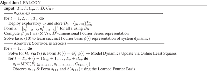
FALCON starts with a short warm-up period to collect some data about the unknown system. In this phase, the goal is to purely explore the system and recover a coarse model of the dynamics. Therefore, FALCON focuses on safely exciting the system for Tw time steps. The predominant choice for such a task is to use isotropic Gaussian inputs, ({u}_{t} sim {mathbf{N}}(0,{sigma }_{u}I)). However, for certain tasks, one may require smoother or safer exploration. This is usually the case in safety-critical control tasks like flight control under turbulence35 or bipedal/quadrupedal walking71. In these situations, FALCON can use time-correlated inputs for smooth actions such that it avoids jerky and sudden changes in the actions. To this end, for some γ ∈ [0, 1], FALCON can use the following control inputs
where ({{boldsymbol{eta }}}_{t} sim mathbf{N}(0,{sigma }_{eta }I)). We deploy this controller with γ = 0.8 during the warm-up phase in our experiments. Moreover, FALCON can deploy known safe nominal controllers, such as trajectory generators72 or PID controller, accompanied with isotropic excitements, i.e., ut = K(yt) + ηt where K( ⋅ ) is the nominal controller and ({{boldsymbol{eta }}}_{t} sim {mathbf{N}}(0,{sigma }_{eta }I)).
After the warm-up, FALCON starts adaptive control of the underlying system. It uses epochs of doubling length starting with an initial epoch of tep time steps, i.e., each ith epoch is 2i−1tep time steps for i = 1, 2, . . . . FALCON is a single trajectory algorithm and does not require a reset between epochs. This makes FALCON efficient in data collection in the experiments.
At the end of the warm-up, FALCON estimates the model dynamics as a linear model in Fourier basis. To this end, it generates Tw − h + 1 subsequences of h input-output pairs,
for h ≤ i ≤ Tw. Using (1), one can write the system dynamics as yt = F(st) + et. To estimate the unknown nonlinear function F, FALCON considers the nth order Fourier expansion of F and generates D-dimensional Fourier series representations of all st as given in (6), ϕ(st). The order of the Fourier expansion, thus the dimension D, is an important hyperparameter of FALCON. This choice depends on many factors including prior knowledge of the system dynamics, the difficulty of the learning task, and the computational budget. As explained in the Overview section of Methods, a wide range of nonlinear systems can be represented as linear models in the Fourier basis. Therefore, FALCON considers the following model for estimating the system dynamics F,
for an unknown ({Theta }_{* }in {{mathbb{R}}}^{Dtimes {d}_{y}}). To recover an estimate of Θ* solves a least-squares problem,
for some λ > 0, where ({Y}_{t}=[{y}_{t},…,{y}_{h}]in {{mathbb{R}}}^{{d}_{y}times t-h+1},{Phi }_{t}=[phi ({s}_{t}),…,phi ({s}_{h})]in {{mathbb{R}}}^{Dtimes t-h+1}). The solution to this problem is given as ({hat{Theta }}_{1}={({Phi }_{{T}_{w}}{Phi }_{{T}_{w}}^{top }+lambda I)}^{-1}{Phi }_{{T}_{w}}{Y}_{{T}_{w}}^{top }.) Using ({hat{Theta }}_{1}), FALCON estimates the system dynamics as ({hat{F}}_{1}(s)={hat{Theta }}_{1}^{top }phi (s).) FALCON repeats this dynamics estimation process at the beginning of each epoch using all the data gathered so far. Note that for large D, computing the closed-form solution could be computationally demanding or cause numerical errors. Instead, the model estimates can be updated recursively throughout the epochs using online updates, which we utilize in our implementation for the experiments. In particular, FALCON stores only the current model estimate, i.e., the model estimate at time step t in epoch i: ({hat{Theta }}_{i,t}), and the inverse design matrix (sample covariance matrix), i.e., ({V}_{t-1}^{-1}={({Phi }_{t}{Phi }_{t}^{top }+lambda I)}^{-1}). Using these the model estimates can be updated recursively throughout the epochs using online or batch updates via
where ({V}_{t-1}^{-1}) is also updated recursively73,
Note that FALCON uses the initial most recent model estimate at the beginning of the epoch for the control design during the entire epoch. These online update rules are used to efficiently update the model estimates in the background at each time step with the new data such that at the beginning of the next epoch, there is no delay in updating the model estimate. This feature is important in real-time control systems where any delay in the system can cause further problems and compromise safety.
Note that as the order of the Fourier basis increases, D increases exponentially in the system’s dimension. For large h, i.e., higher order NARX models, this may cause an additional computational burden. To remedy this, we propose to use ℓ1-constrained Fourier basis and Least Absolute Shrinkage and Selection Operator, i.e., lasso42, for an improved basis selection in FALCON after the warm-up period. In particular, instead of generating the bases ωis for all n, we only consider the ℓ1-constrained bases, i.e., ∥ωi∥1 ≤ n. The ℓ1 constraint reduces the number of basis vectors from (1+2{n}^{h({d}_{y}+{d}_{u})}) to (2{D}^{{prime} }) basis vectors where
We then solve the lasso problem for the warm-up samples that are represented in these ℓ1-constrained Fourier basis vectors. Lasso is the ℓ1-regularized least squares method to recover sparse models, with few non-zero coefficients. Given the data points gathered during the warm-up period (T_w), using ({D}^{{prime} }) number basis vectors with ∥ωi∥1 ≤ n, FALCON forms the following feature representations for ({s}_{h},ldots ,{s}_{{T}_{w}}) generated via (T_w):
FALCON then solves the lasso problem:
for some α > 0. FALCON then uses the basis vectors that have nonzero feature coefficients (entries) in the solution of (10), W⋆, for learning the model dynamics in the adaptive control phase. The choice of α determines the sparsity of the model learned W⋆ which in turn determines the number of basis vectors, D, used in model learning, i.e., bigger α results fewer non-zero entries in W⋆ and fewer basis vectors for estimating the dynamics in the adaptive control period. This improved basis selection significantly decreases D and reduces the computational burden and the samples required to learn the dynamics.
Once FALCON has an estimated model, it uses an MPC policy to design the control inputs during the epoch. The choice of the MPC policy depends on the control task. In general, the MPC policies are either optimization-based48 or sampling-based49. However, sampling-based methods are usually preferred in model-based RL due to challenging nonlinear system dynamics and complicated cost functions50. Thus, FALCON uses Cross-Entropy Method (CEM) as the MPC policy. CEM is a sampling-based (zeroth order) MPC policy to solve the problem given in (3). CEM maintains a distribution, predominantly Gaussian, to sample action roll-outs for the planning horizon and iteratively updates this distribution to assign a higher probability near lower-cost action sequences based on the estimated dynamics. After a certain number of updates (once it converges), it executes the first action on the lowest cost-achieving action sequence in the sampled roll-outs. The CEM algorithm is given in full detail in Algorithm 2.
Algorithm 2
Cross Entropy Method (CEM)
1: Input:(tau ,K,M,0 < gamma < 1,N,{sigma }_{init},hat{F}(cdot ),{y}_{t:t-h+1},{u}_{t-1:t-h+1},{C}_{t:(t+tau -1)},{mathbf{N}}(mu ,{sigma }^{2}I))
2: for i = 1, 2, …, M do
3: if i = 1 then
4: Set the mean μ to the best action sequence from the previous time-step by shifting (Warm-Start)
5: Set the variance σ = σinit
6: Sample Kγi−1 action sequences ({u}_{t:t+tau -1}^{j}) of τ length using ({mathbf{N}}(mu ,{sigma }^{2}I),jin {1,ldots ,K{gamma }^{i-1}})
7: Compute the trajectory roll-outs (forall {u}_{t:t+tau -1}^{j}) using (hat{F}(cdot )) with initial yt:t−h+1, ut−1:t−h+1
8: Compute the cost of each trajectory roll-out using Ct🙁t+τ−1)
9: Sample best N action sequences according to their acquired costs
10: Update μ and σ to fit the Gaussian distribution to the best N action sequences
11: Execute the first action of (i) the best action sequence of the Mth iteration or (ii) a newly sampled action sequence using ({mathbf{N}}(mu ,{sigma }^{2}I))
At any time step t, FALCON uses the most recent dynamics estimate ({hat{F}}_{k}(cdot )), the last h input-output pairs as the initial condition, and the next τ cost functions Ct🙁t+τ) in solving the problem in (3) for the planning horizon τ. FALCON executes the first action ut in the solution of (3), receives the output yt+1, and constructs st+1 and ϕ(st+1). FALCON repeats this adaptive control process throughout the epoch. Note that any safety or physical constraint can be easily included in the MPC policy design problem (3), which makes FALCON a reliable algorithm for safety-critical environments.
Implementation details of FALCON
We use an order-4 NARX model for learning the underlying system dynamics, h = 4. In our experiments, we deduce that this is optimal to overcome the uncertainties of partial observability and reasonable computational complexity. With this choice, st in the system modeling becomes 44-dimensional vector. To estimate the unknown nonlinear system F, we consider the 3rd order Fourier expansion. However, to reduce the computational complexity for such a high-dimensional learning problem, we only use ∥ωi∥1 ≤ 3 constrained basis vectors and use lasso to identify the most relevant basis vectors using the warm-up data as described in Appendix. At the end of this procedure, we obtain D = 319 dimensional Fourier series representation for learning the model dynamics.
The control goal in disturbance rejection is to minimize the mean and the standard deviation of the lift forces acting on the airfoil. Thus, we design our cost function to penalize large lift forces, rapid changes in lift forces, and fast/jittery action changes. FALCON has a warm-up duration of around 35 s, i.e., Tw = 1500 samples, using the time-correlated sum of Gaussian inputs for smooth exploration to collect some data about the unknown system dynamics and recover the most relevant Fourier basis. The epochs of the adaptive control period are approximately 38 seconds, tep = 1600 samples per epoch. FALCON uses Cross-Entropy Method (CEM) as the MPC policy. CEM is a sampling-based MPC policy to solve the problem given in (3)49. CEM maintains a distribution, predominantly Gaussian, to sample action roll-outs for the planning horizon and iteratively updates this distribution to assign a higher probability near lower-cost action sequences based on the estimated dynamics. After a certain number of updates, it executes the first action on the lowest cost-achieving action sequence in the sampled roll-outs. The CEM algorithm is given in full detail in Algorithm 2.
We compare FALCON with several model-free RL methods, including TD355, LSTM-TD356, SAC57, and the industry-standard responsive control strategy of PID (Proportional-Integral-Derivative) controller. Of all these algorithms, LSTM-TD3 has been demonstrated to achieve state-of-the-art performance in disturbance rejection35. Unlike FALCON, the model-free methods work in episodes with reset for retraining. We train the model-free methods for 200 episodes of 800 samples per episode and test the best-performing policy in presenting the results. All methods, including FALCON, are implemented with 42 Hz sensing and control frequency.
Adaptive control design
FALCON uses CEM as the MPC policy. CEM is a sampling-based (zeroth order) MPC policy to solve the problem given in (3)49. CEM maintains a distribution, predominantly Gaussian, to sample action roll-outs for the planning horizon and iteratively updates this distribution to assign a higher probability near lower-cost action sequences based on the estimated dynamics. After a certain number of updates (once it converges), it executes the first action on the lowest cost-achieving action sequence in the sampled roll-outs. For the planning horizon, FALCON uses τ = 5 in CEM. Furthermore, FALCON samples K = 1000 trajectories in the first action roll-out of CEM and decays the number of samples in each update. In prior works, this sampling strategy has been observed as an efficient way to avoid possible local minima in finding the optimal action actions66. The CEM algorithm is given in full detail in Algorithm 2.
Table 2 summarizes the hyperparameters for FALCON in our experiments. In order to achieve the desired control and sensing frequency number of CEM samples (K) and iterations (M) create a trade-off in the implementation. Maintaining this control and sensing frequency is crucial in order to avoid undersampling the turbulent dynamics.
Stability and performance guarantees
-
1.
We derive the learning guarantees for using the Fourier series as a basis for learning the dynamics. In particular, we prove that FALCON learns any partially observable nonlinear system that belongs to an extended Sobolev space of periodic functions with the near-optimal estimation error rate of (tilde{O},({T}^{varepsilon -0.5})), after T samples where ε depends on the smoothness of the Sobolev space and 0 ≤ ε < 0.5.
-
2.
We show that FALCON attains (tilde{O},(sqrt{T})) regret against the agent who has access to the underlying dynamics and uses the same control design. To the best of our knowledge, FALCON is the first efficient RL algorithm that achieves (tilde{O},(sqrt{T})) regret in online control of nonlinear dynamical systems, Table 3.
Most of the model-based RL methods with guarantees are developed for linear systems due to their simplicity74,75,76,77,78,79,80,81,82. The central goal of these works is to derive finite-time learning and regret guarantees. Recently, there has been a growing interest to extend these results to nonlinear systems.83,84 consider the model learning problem by modeling the underlying system as a linear function of a known nonlinear basis.85 study the regret minimization in this setting and propose an approach which attains (tilde{O},(sqrt{T})) regret, but is not computationally or memory efficient.63 use kernel approximation to learn the underlying system and design an efficient RL algorithm, yet, achieve (tilde{O},({T}^{2/3})) regret. Further, the empirical performances of these methods are demonstrated only on simulation. FALCON provides significant improvements upon these prior works in terms of regret guarantee and efficiency (Table 3). To the best of our knowledge, FALCON is the first efficient RL algorithm to attain (tilde{O},(sqrt{T})) regret in partially observable nonlinear systems and achieve effective performance in a challenging real-world task.
In this section, we provide the learning and regret guarantees of FALCON. The technical details and the proofs are given in Supplementary Material. First, let ({F}_{i}(cdot ):{{mathbb{R}}}^{h({d}_{y}+{d}_{u})}to {mathbb{R}}) denote the ith mapping of F from input to output, i.e., yt,i = Fi(st) + et,i. We assume the following regularities on the system.
Assumption 1
The system F( ⋅ ) is L-Lipschitz and (λ, α, K)-exponentially input-to-output stable (e-IOS), i.e.,
for t > t0, λ, K > 0 and 0 < α < 1. Moreover, Fi (or its periodic extension) lives in ({W}_{p}^{m,2}({[0,2pi ]}^{h({d}_{y}+{d}_{u})})), for all 1 ≤ i ≤ dy.
This assumption is inspired by the chaotic nature of the systems that indicate a fast transitory phase from their earlier states, making the current dynamics forget the much earlier states. Please note that if the system dynamics show complex behavior that does not satisfy this assumption, the method introduced in this work is no longer directly applicable. The first assumption is required to avoid blow-ups in the output due to noise and unmodeled dynamics. The Sobolev space assumption guarantees that the underlying system can be represented on the Fourier basis. For simplicity, we assume that ({e}_{t} sim {mathbf{N}}(0,{sigma }_{e}^{2}I)), yet our technical results hold for sub-Gaussian noise. Finally, we have the following property on the cost Ct( ⋅ , ⋅ ).
Assumption 2
For any (y,{y}^{{prime} }) and (u,{u}^{{prime} }) such that (max {parallel y-{y}^{{prime} }parallel ,parallel u-{u}^{{prime} }parallel }le Gamma) and ({B}_{uy}=max {parallel yparallel ,parallel uparallel }), for all (t,| {C}_{t}(y,u)-{C}_{t}({y}^{{prime} },{u}^{{prime} })| le R(parallel y-{y}^{{prime} }{parallel }^{2}+parallel u-{u}^{{prime} }{parallel }^{2})) and (0le {C}_{t}(y,u)le R{B}_{uy}^{2}).
The regret of FALCON is computed with respect to the policy π⋆ that uses the same MPC policy at each time step with the true transition dynamics F in the control design. Thus, the goal of FALCON is to minimize ({bf{Regret}}(T)=mathop{sum }nolimits_{t = 1}^{T}({C}_{t}({y}_{t},{u}_{t})-{C}_{t}({y}_{t}^{{pi }_{star }},{u}_{t}^{{pi }_{star }}))). For consistent and reliable initial estimation of the underlying system, we assume that FALCON uses bounded persistently exciting inputs during the warm-up period. Given these inputs, we have the following learning guarantee.
Proposition 3
Let ({alpha }_{m}=mathop{sup }nolimits_{i,parallel sparallel le S}parallel {partial }^{m}{F}_{i}(s){parallel }_{{L}^{infty }}) and d = h(dy + du). Using nth order Fourier basis for learning the model for sufficiently large n, after the warm-up of Tw, with high probability (mathop{sup }nolimits_{parallel sparallel le S}parallel F(s)-hat{F}(s){parallel }_{infty }=tilde{{O}},({n}^{d}{T}_{w}^{-0.5}+{alpha }_{m}{n}^{-m})).
Here (tilde{O},(cdot )) presents the order up to logarithmic terms. The proof is given in Supplementary Material, where we use standard least-squares estimation error analysis and the multivariate analog of Jackson’s theorem for trigonometric polynomial approximation86. This result shows that the underlying system can be identified with the optimal rate of (1/sqrt{T}), yet, due to the properties of the underlying system, there exists a constant term in the estimation error. Note that this constant term depends on the smoothness of the system. For nonlinear systems that live in high-order Sobolev spaces m, this constant term can be small. In the extreme case of infinitely differentiable systems, this constant term approaches to 0. Thus, we have (mathop{sup }nolimits_{parallel sparallel le S}parallel F(s)-hat{F}(s){parallel }_{infty }=tilde{{{O}}},({T}_{w}^{varepsilon -0.5})) after warm-up, where ε depends on the smoothness of the system and the order of Fourier basis. Next, we focus on the adaptive control task. We have the following assumption on the MPC policy that FALCON deploys.
Assumption 4
The MPC policy with F( ⋅ ) achieves e-IOS, i.e., (forall t, >, {t}_{0},parallel {y}_{t}parallel le {(1-rho )}^{t-{t}_{0}}parallel {y}_{{t}_{0}}parallel +M{sup }_{iin [{t}_{0}:t]}parallel {e}_{i}parallel), for M > 0 and 0 < ρ < 1. The MPC policy with planning model (hat{F}(cdot )), such that (mathop{sup }nolimits_{parallel sparallel le S}parallel F(s)-hat{F}(s){parallel }_{infty }le epsilon), achieves e-IOS with ρ/2 and 2M and synthesizes persistently exciting inputs which are locally Lo-Lipschitz in planning model.
This assumption states that MPC stabilizes the underlying system by using any model within a neighborhood around the underlying system for planning. This assumption is mild and one can show that it holds for linear systems. Intuitively, this assumption holds for nonlinear systems with valid linearization for bounded inputs. Finally, the last statement allows consistent estimation during the adaptive control with reasonable variations in the input due to model dynamics used in planning. In practice, this condition is usually satisfied by the combination of unmodelled system dynamics, system noise, and sampling-based MPC policies63. Note that for a long enough warm-up Tw, the model estimation error can be made small enough to achieve stabilization via the MPC policy. Once FALCON is guaranteed to stabilize the dynamics, it safely regulates the system.
Theorem 5
Suppose Assumptions 1, 2, and 4 hold. Let Tw be chosen long enough such that the MPC policy of FALCON stabilizes the underlying system dynamics. Then, with high probability, for large enough T, FALCON attains regret of ({bf{REGRET}}(T)=tilde{{O}},(sqrt{T}+{epsilon }^{{prime} }T)), where ({epsilon }^{{prime} }) depends on the smoothness of the underlying system. For sufficiently smooth systems, it achieves ({bf{REGRET}}(T)=tilde{{O}},(sqrt{T})).
The proof is given in Supplementary Material. This shows that FALCON is the first efficient RL algorithm that attains (tilde{{O}},(sqrt{T})) regret in adaptive control of partially observable nonlinear systems. Note that this result applies to various systems that are governed by partial differential equations since FALCON only requires the periodic extension of the model dynamics to live in the Sobolev space of periodic functions. Moreover, for infinitely smooth systems, e.g. sinusoidal systems, one can improve Proposition 3, and this in turn would give significantly improved regret upper bound for FALCON.
Corollary 6
Under the setting of Theorem 5, for an infinitely smooth system, i.e., ({F}_{i}in {W}_{p}^{infty ,2}({[0,2pi ]}^{h({d}_{y}+{d}_{u})})) for 1 ≤ i ≤ dy, with high probability, FALCON attains REGRET(T) = polylog(T).
This shows that for a certain class of dynamical systems, using the domain knowledge on the system dynamics, FALCON can achieve almost logarithmic regret even if the underlying system is unknown.
Wing system design and manufacturing
The wing system was designed with a standard NACA0012 airfoil shape, which was previously studied for its dynamics in a bluff-body wake at a similar Reynolds number35,87. The modular wing body was 3D printed using a combination of materials, allowing for various sensor configurations. The central module, made of micro carbon fiber-filled nylon (Markforged Onyx) reinforced with carbon fibers for added strength and rigidity, housed the primary electronics and secured the system to its mounting via a sweptback fairing. Spanwise sections designed to house individual pressure sensors were also printed using carbon fiber-filled nylon. Clear PLA was used to print the sections between the sensors, which were aligned and connected using carbon fiber spars to add rigidity. Trailing edge flaps were cut from insulation foam and covered with an adhesive-backed coating for protection and improved surface finish.
The wing had a spanwise length of 1 m and a total chord length of 25 cm with 5 cm trailing edge flaps. Using the mean flow velocity near the leading edge, the system had a Reynolds number of approximately Re ≈ 110,000. There were 9 sensor locations distributed symmetrically about the wing, with exactly 10cm between each location. The central sensor location featured a pitot-static tube, with the rest of the sensor locations featuring surface pressure taps. The pressure taps and the pitot-static tube were printed using an SLA printer (Formlabs Form3) for improved surface feature accuracy. Pressure taps were located at 0.4%, 0.7%, 1.5%, and 6% of the chord length from the leading edge on both the pressure and suction sides of the wing. The fairing on which the wing was mounted was reinforced with carbon fiber and aluminum and was set back with an angle of 60o to reduce aerodynamic interactions between the fairing and the wing. The fairing was connected to a set of vertically-aligned air bearings (New Way), which allowed for nearly frictionless motion along a single axis while constraining all other directions. The constrained fairing was mounted directly to a single-axis load cell (Interface SM-50) that passed the signal through an amplifier (Interface Model SGA) with a 50 Hz low pass filter, and the signal was read by a DAQ (NI USB-6008).
The wing had a total of 9 ultra-low range digital pressure sensors (Honeywell RSCDRRM2.5MDSE3) to measure pressure values, which were communicated with a microcontroller (Teensy 4.0). The microcontroller also controlled the high-speed brushless servo motors (MKSHBL6625) that drove the trailing edge flaps. Due to mechanical restraints, the actuation for the servo motors had a maximum/minimum position of + 40o/ −40o. Both the microcontroller and the DAQ communicated with a desktop computer, which received measurements and sent actions. The full control loop operated at approximately 42 Hz.
Generation and characterizations of turbulence
The John W. Lucas Wind Tunnel (LWT) at Caltech was used to conduct all quantitative experiments discussed in this study. The wind tunnel is a closed-loop design with a test section size of 130 cm × 180 cm. To generate turbulence, an asymmetric bluff body was mounted to the wind tunnel using bungee cords, creating a wake of irregular and turbulent flow. The bluff body consisted of a large diameter cylinder (30 cm) with an asymmetrically mounted flat plate at the front, giving the entire body an effective diameter of 53 cm (Fig. 1C). To encourage vortex dislocation and add irregularity to vortex shedding, the cylinder spanned the full width of the tunnel, while the flat plate only had a width of 60 cm. The bluff body was positioned 170 cm upstream of the wing system, with a vertical offset of 48 cm, and sparse elastic bands were placed horizontally across the test section immediately upstream of the bluff body to further increase turbulence intensity.
We used particle image velocimetry (PIV) (Fig. 3) to visualize a limited portion of the bluff body wake. PIV is a quantitative flow visualization technique capable of measuring the velocity fields of fluid flows88. Here we performed two-dimensional, two-component (2D2C) PIV. This involves using a laser sheet to illuminate small, dense, neutrally buoyant seed particles. Recording the illuminated particles with a high-speed camera, we can estimate velocity fields by calculating the effective inter-frame displacement of groups of particles via cross-correlation of subsequent images. Performing these experiments in air, we used a 200 mJ/pulse dual pulsed laser (Lumibird Evergreen) to illuminate soap bubbles (15-micron mean diameter) generated with a custom-built bubbler. The flow was recorded with a 4 MP CCD camera (IMPERX Bobcat B2401).
Characterization of the flow near the wing system was performed using a hot-wire anemometer (TSI IFA-300). The anemometer was mounted approximately 2 cm upstream of the leading edge of the airfoil, and measurements were taken at 1000 Hz for 120 s. The turbulence intensity was determined to be 10.8% using the hot-wire anemometer. We found the dominant shedding frequency to be 2.44 Hz, although as mentioned above our oscillating bluff body encouraged irregularities in the shedding process.
Baseline algorithms
In our experiments, besides FALCON, we test several model-free RL methods, including Twin Delayed DDPG (TD3)55, LSTM-TD356, Soft Actor-Critic (SAC)57, and the industry-standard responsive control strategy of PID controller. Of all these algorithms LSTM-TD3 has recently demonstrated to achieve state-of-the-art performance in predictive flow disturbance rejection35. Note that both TD3 and LSTM-TD3 provide deterministic policies, whereas SAC designs stochastic policies. Unlike FALCON, these model-free methods work in episodes where the algorithms stop retraining the policy parameters (reset). We train the model-free methods for 200 episodes of 800 samples per episode and test the best-performing policy in presenting the results. The full 200 episodes of training for the best-performing policy in each method are shown in Fig. 5. All methods were implemented using an NVIDIA GeForce RTX 3070 which enabled a 42 Hz frequency for sensing and control. The brief descriptions of the algorithms are given below with the relevant hyperparameters in Tables 4–7.
TD3 is a deterministic actor-critic type RL framework that builds on previous value-based methods. TD3 injects noise into actions to enable policy exploration (i.e., exploration noise), and injects noise into critic updates to regularize and smooth the resulting policy (i.e., policy smoothing noise). TD3 also uses delayed policy updates which decreases variance in value estimates. For this work, we added gradient clipping to both actor and critic networks to encourage more stable learning in a real-world setting. TD3 has been proven effective in several simulated55 environments and has previously been used for experimental flow control in a different setting34. For further implementation details of TD3 please refer to55 and the code provided in the submission.
LSTM-TD3 uses the same fundamental algorithm as TD3 but includes LSTM cells for a recurrent actor-critic framework. It was modified from TD3 to better address problems suffering from partial observability56. For further implementation details of LSTM-TD3 please refer to56 and the code provided in the submission.
The Soft Actor-Critic (SAC) method is based on the maximum entropy RL framework that wants to maximize the performance/reward concurrently maximizing the entropy of the policy, i.e., increase the randomness in the policy. Intuitively, this method results in a stochastic policy that achieves good performance and provides the most randomness in achieving this result. SAC uses a temperature parameter to weigh the entropy term relative to the reward function. The ideal temperature parameter can be automatically learned during training. This method is initially proposed for real-world robotic learning to facilitate smooth exploration, tolerate unexpected perturbations/changes during execution, and improve robustness to hyperparameters and sample efficiency. To this end, it requires relatively less hyperparameters compared to other model-free RL methods. For further implementation details of SAC please refer to57 and the code provided in the submission.
PID control is the most prevalent method found in industrial and commercial applications. PID controllers use a basic feedback control loop that attempts to minimize the error between an observed value and a desired setpoint. PID controllers weigh a proportional term, an integral term, and a derivative term, all of which are tuned for each specific application. As the name suggests, the proportional term contributes a control signal that is directly proportional to the magnitude of the error. The integral term provides a signal that corresponds to the running accumulated error but is slow to react. The derivative term sends a control signal that is proportional to the error rate of change, which effectively smooths behavior. All three of these terms are weighed through corresponding constant values (i.e., KP, KI, KD) that can be found through various tuning methods. For further implementation details of PID please refer to the code provided in the submission.
Responses