Fast, scale-adaptive and uncertainty-aware downscaling of Earth system model fields with generative machine learning

Main
Accurate and high-resolution climate simulations are of crucial importance in projecting the climatic, hydrological, ecological and socioeconomic impacts of anthropogenic climate change. Precipitation is one of the most important climate variables, with particularly large impacts, for example, on vegetation and crop yields, infrastructure or the economy1. However, it is also the variable that is arguably the most difficult to model and predict, especially extreme precipitation events, resulting from a complex interaction of processes over a large range of spatial and temporal scales that cannot be fully resolved.
Numerical Earth system models (ESMs) are our main tool to project the future evolution of precipitation and its extremes. However, they exhibit biases and have much coarser spatial resolution, on the order of 10–100 km, than that needed for the reliable assessments of impacts of climate change2. Therefore, ESM projections have to be downscaled to higher resolution, for which several machine-learning-based approaches have recently been proposed. Due to the chaotic nature of geophysical fluid dynamics, the trajectory of climate simulations will not match historical observations, requiring approaches suitable for unpaired samples to learn such tasks. Recently, methods from generative deep learning have shown promising results in downscaling or correcting spatial patterns of ESM simulations. Normalizing flows (NFs)3 and generative adversarial networks (GANs)4 can perform these tasks efficiently in a single step5,6,7,8,9,10. However, NFs often exhibit lower quality, for example, less sharp and less detailed generated images, whereas GANs can suffer from training instabilities and problems such as mode collapse11. Moreover, these approaches require computationally expensive retraining of the neural networks for each specific ESM simulation to be processed. This makes downscaling large ESM ensembles, as needed in impact assessments, prohibitively costly and time-consuming.
Diffusion-based generative models have demonstrated superior performance over NFs and GANs on classical image generation tasks12,13. Crucially, iteratively solving the reversed diffusion equation allows for strong control over the image sampling process.
This enables foundation models for computer vision and image processing, which are only trained to generate target dataset samples from noise and which can later be repurposed for different downstream tasks, for example, inpainting, classification, colourization or generating realistic images based on a given ‘stroke sketch’ guide as with SDEdit14,15,16.
So far, such diffusion-model-based approaches have only been applied to downscale idealized fluid dynamics17,18 in Earth system science-related tasks. Both studies use stochastic differential equation (SDE)-based diffusion models and achieve remarkable performance. The iterative integration of the SDE, however, implies that the generative network needs to be evaluated up to 1,000 times to downscale a single simulated field. This makes such methods unsuitable for processing large simulation datasets, for example, at high temporal resolution or over long periods, as would be needed in the context of climate change projections and impact assessments.
Much effort has been taken to improve the sampling speed of diffusion models. Using ordinary differential equations instead of SDEs can reduce the number of integration steps to around 10–50 (refs. 19,20). Distillation techniques can also be applied to improve the sampling speed to a single step21,22. However, they require additional training costs and hyperparameter choices. In general, a trade-off between the number of generative steps and the resulting image quality scores has been found13,20. Recently, consistency models (CMs) have been proposed that can be directly trained as single-step generative models without sacrifices in the controllability of sampling23. CMs have been shown to outperform distilled single-step diffusion models on common image benchmarks23.
In this work, we tackle the shortcomings of standard diffusion models by using CMs23 to downscale global precipitation simulations from three different ESMs in a single step (Fig. 1). In summary, we aim to establish a generative model for downscaling ESM fields that fulfils the following conditions:
-
The CM model is trained on the target dataset only, without conditioning on the ESM. This makes the method applicable to any ESM without requiring computationally expensive retraining.
-
The training minimizes a regression loss that is more stable than the adversarial training in previous methods6,7,9,10.
-
The generative downscaling is controllable at the inference stage after training, allowing the choice of a characteristic spatial scale up to which unbiased spatial patterns are preserved in the ESM.
-
The model only requires a single network evaluation instead of the many iterative evaluations in diffusion-model-based downscaling approaches17,18.
-
The model allows to generate a large number of downscaled realizations for a single ESM field (that is, a one-to-many mapping), enabling probabilistic downscaling and a quantification of the sampling spread.
-
The method does not require specifically formulated physical constraints24 to preserve trends9.

Unconditional training of score-based diffusion and CMs that learn to reverse a forward diffusion process (i). Although the SDE of the diffusion model requires an iterative integration over many steps, the CM only takes a single step to generate a global precipitation field from noise. The unconditionally trained CM is used to downscale (upsample) a low-resolution ESM precipitation field to a four times higher resolution (ii). By adding noise of a chosen variance to the ESM field, the spatial scale to be preserved in the ESM can be controlled: a small noise variance implies a close pairing to the original ESM field with only small changes; a larger variance will result in changes at larger spatial scales and in weaker pairing to the ESM field.
Results
We evaluate our CM-based downscaling method against an SDE bridge17 over the test-set data. We investigate the performance of downscaling, the ability to correct distributional biases in the ESM, the sample spread given a chosen spatial scale and the preservation of trends in future climate scenarios.
Downscaling spatial fields
For a qualitative comparison, we show single precipitation fields in Fig. 2. Both generative downscaling methods, based on the SDE bridge (Fig. 2e) and CM (Fig. 2g), can produce high-resolution precipitation fields that are visually indistinguishable from the unpaired ERA5 field (Fig. 2a). A similar performance can be seen when downscaling simulations from the state-of-the-art GFDL-ESM4 and the more lightweight SpeedyWeather.jl general circulation model, as well as when applying our method to initially upscaled ERA5 data as a proof of concept (Supplementary Figs. 3 and 6).
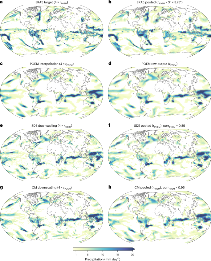
a, Daily precipitation from the ERA5 target dataset was used for training the generative models. b, Same data as a, but at four times lower resolution for comparisons. c,d, Precipitation field from a historical run of the POEM ESM interpolated to the target resolution (c) and on its native resolution of 3° × 3.75° (d). The POEM fields are unpaired with the ERA5 field from the same date or any other ERA5 field. e, The downscaled field from POEM (d) using the SDE bridge method (d→e). f, An upscaled (average pooled) representation of e for comparison with the original POEM field is shown in d and the Pearson correlation between the two. g,h, Downscaling POEM with the CM-based method (d→g), and the respective pooled field (h). Note that the CM downscaling yields a higher correlation and, hence, better consistency of the large-scale features than the SDE method.
When upscaled back to the native ESM resolution using a 4 × 4-kernel average pooling, an accurate representation of the low-resolution ESM simulation field is apparent. As indicated in Fig. 2f,h, for the case of the Potsdam Earth Model (POEM) model, a high Pearson correlation of 0.89 and 0.95 for the SDE and CM methods, respectively, is maintained between upscaled corrected and native fields. We provide correlation statistics for the entire test set in Table 1. Besides the average pooled fields, we also compare the downscaled and linearly interpolated POEM simulation on the high-resolution grid by applying a low-pass filter with a cut-off frequency set to k* = 0.0667 on the downscaled fields before computing the correlation. In this way, we test the preservation of the large-scale patterns in the ESM. More specifically, we measure how similar the downscaled fields are to the original coarse fields when upscaling them back to the same resolution. The SDE bridge achieves a mean correlation of 0.918 and 0.916 for the average pooled and low-pass-filtered fields, respectively. Our CM-based method achieves even higher correlation values of 0.954 and 0.941 for the corresponding measures. The CM-based downscaling also shows higher correlations when downscaling ERA5 (Supplementary Table 2).
We estimate the average time it takes to produce a single sample with the SDE and CM methods on an NVIDIA V100 32 GB graphics processing unit. The average is taken over 100 samples. We set the number of SDE integration steps to 500 (ref. 17), which is lower than the typical 1,000–2,000 steps12,13. The SDE takes an average of 39.4 s, whereas the CM samples are much more efficient, taking only 0.1 s, scaling linearly with the number of samples.
We analyse the downscaling performance of the CM and SDE bridge approaches quantitatively using power spectral densities (PSDs)10,25. The interpolated ESM fields under-represent variability at small spatial scales, because these are not present in the low-resolution simulation. This implies an underestimation of spatial intermittency, that is, overly smooth precipitation patterns, which is highly problematic for impact assessment. The generative downscaling methods based on SDEs and CM perform very well in increasing spatial resolution and greatly improve the spatial intermittency at smaller spatial scales (Fig. 3a). The PSD improvements are found to be consistent when applying the CM downscaling to the GFDL-ESM4 and SpeedyWeather.jl simulations (Supplementary Fig. 4).
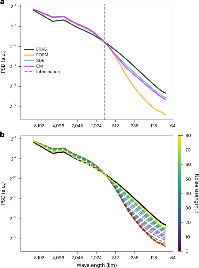
a, Comparison of the PSDs for the target ERA5 reanalysis data (black), the POEM simulations interpolated to the same high-resolution grid (orange), the SDE bridge (cyan) and the CM downscaling (magenta). The vertical dashed lines mark the spatial scale at which the PSDs of POEM and ERA5 intersect and are, thus, a natural choice for the wavenumber k* up to which to correct, which, in turn, determines t*—the noising strength in the diffusion models (equation (11)). b, CM downscaling (dashed lines) applied to be consistent with different spatial scales as a function of noising strength t over the entire range [tmin, tmax]. Noising small scales implies nearly reproducing the POEM simulations, whereas noising larger scales corresponds to a weaker pairing to the ESM (Fig. 1).
We also investigate the change in PSDs as a function of the noise variance schedule time t (Fig. 3b), which is directly related to the spatial scale up to which patterns are corrected (Methods). For minimal noise, that is, t* = tmin, the CM model reproduces the PSD of the ESM, as expected from equation (5) because there are no changes made to the ESM field. For maximal variance with t* = tmax, the PSD closely matches the ERA5 reanalysis ground truth. For any tmin < t* < tmax, we find a trade-off between the two extreme cases that match the PSD above and below the intersection (Fig. 3a, dotted grey line) to a certain degree, depending on the spatial scale preserved in the ESM.
To test the temporal consistency of the downscaled fields, we report temporal autocorrelation values computed for each grid cell as global averages (Supplementary Fig. 8). We find that the generative and stochastic SDE and CM methods result in a more accurate temporal correlation than the deterministic approach of quantile mapping and bilinear interpolation.
Bias correction
We compare the ability to correct biases in the ESM with histograms of relative frequency and latitude profiles of mean precipitation to investigate the reduction in known biases such as double-Intertropical Convergence Zone (ITCZ)26, following the evaluation methodology discussed elsewhere9,10.
When applied to the ESM simulations without preprocessing via quantile delta mapping (QDM)27, the ability of the CM to correct biases naturally depends on the chosen spatial consistency scale (Supplementary Fig. 9). Selecting the smallest scale reproduces the ESM without any changes, thereby inheriting its biases. Choosing the largest possible scales generates samples with statistics very close to the target dataset. However, the fields become increasingly unpaired to the ESM at such high noise levels (Fig. 1). A scale between these two extremes will correct for biases to a varying degree, depending on the chosen correction scale.
In terms of relative frequency histograms, the ESM simulations (without QDM preprocessing) exhibit a very strong under-representation of the right tail of the distribution, that is, of the extremes (Fig. 4a,b). This misrepresentation of extremes is a key problem with existing state-of-the-art ESMs and makes future projections of extreme events and their impacts, as well as related detection and attribution of extremes, highly uncertain.
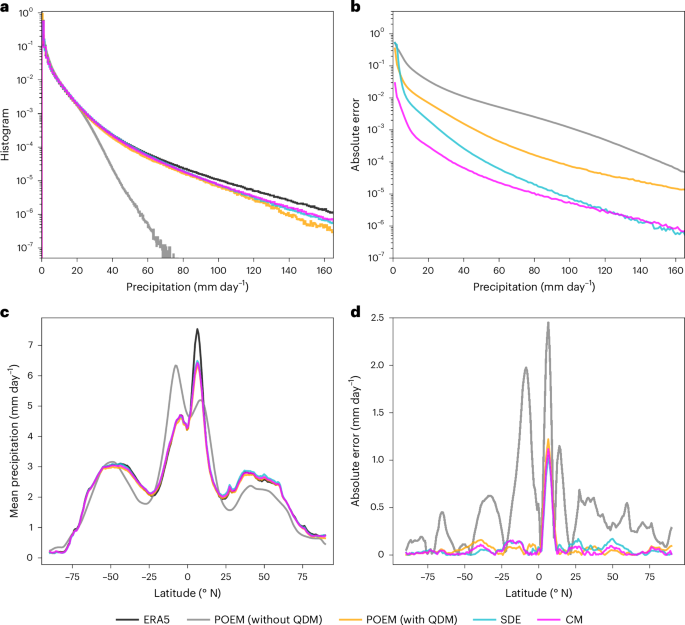
a, Global histograms of relative precipitation frequency for the ERA5 reanalysis data (black), POEM simulations without applying QDM preprocessing (grey), POEM simulations with QDM (orange), the SDE bridge (cyan) and the CM (magenta). b, Absolute errors of the histograms in a with respect to the ERA5 ground truth. c, Precipitation averaged over time and longitudes for the same data as in a. d, Absolute errors of the latitude profile in c. Both SDE and CM downscaling methods are able to further improve on the QDM preprocessing in terms of bias correction, most particularly for extreme precipitation.
Applying QDM to POEM strongly improves the frequency distributions as expected. Downscaling the ESM with the SDE further improves the global histograms by an order magnitude, particularly for the extremes. Our CM-based method shows the overall largest bias reduction in the global histograms (Fig. 4b). When applied to the different ESMs and the upscaled ERA5 data, our method shows a consistent bias correction skill (Supplementary Fig. 5).
We further compute the error in the 95th percentile of the local precipitation histogram for each grid cell and aggregate the absolute value globally (Table 1). The SDE method shows an error of 1.106 mm day–1, reducing the error of the POEM ESM by 68.15%. The CM method performs slightly better with an error of 1.08 mm day–1 and a respective error reduction of 68.92% of the ESM. When downscaling the initially upsampled ERA5 data, the CM again shows better performance, with an error of 0.725 mm day–1 compared with the SDE with an error of 0.868 mm day–1 (Supplementary Table 2).
POEM exhibits a strong double-ITCZ bias that is common among state-of-the-art ESMs26 (Fig. 4c). As expected, QDM can remove most of the biases, though slightly underestimating the peak north of the equator in the ITCZ. The downscaling methods based on the SDE bridge and CM show a similar absolute error for these latitude profiles as when only applying QDM alone (Fig. 4d).
We report the absolute value of the grid-cell-wise error in the long-term mean, again averaged globally, for both downscaling methods (Table 1). The SDE downscaling results in an error of 0.214 mm day–1, reducing the error in POEM by 72.51%, and performing slightly better than our CM method, which exhibits an error of 0.217 mm day–1 and a respective error reduction of 72.08% when applied to POEM. Evaluated on the ERA5 data, we find that the CM method performs slightly better than the SDE in terms of mean absolute error and RMSE (Supplementary Table 2).
Quantifying the sampling spread
Our generative CM-based downscaling is stochastic, with a one-to-many mapping of a single ESM field to many possible downscaled realizations. It, thus, naturally yields a probabilistic downscaling, suitable to estimate the associated uncertainties. By selecting a given spatial scale in the ESM to be preserved by the downscaling method, one automatically chooses a related degree of freedom to generate patterns on smaller scales. Given that our CM method is very efficient at inference, we can generate a large ensemble of high-resolution fields that are consistent with the low-resolution ESM input, and compute statistics such as the sampling spread, which can be interpreted as a measure of the inherent uncertainty of the downscaling task.
We compute an ensemble of 103 downscaled fields from a single ESM precipitation field (Fig. 5a) and evaluate the mean and standard deviation (Fig. 5d,e). The ensemble mean shows close similarity to the ESM simulation interpolated to the same high-resolution grid. The sample spread shows patterns similar to the mean, although with a smaller magnitude.
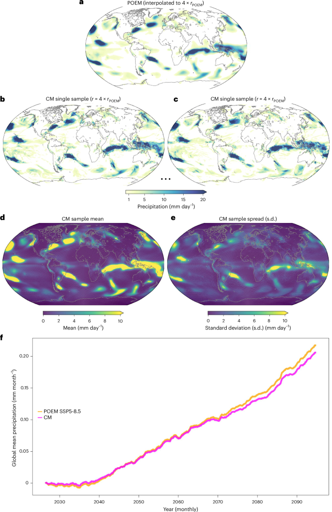
a, ESM field interpolated to the target resolution. b,c, Two different example samples generated by CM downscaling, preserving large-scale patterns and generating new patterns on smaller scales. d,e, Ensemble mean of 103 samples (d) and the standard deviation (e). f, Three-year rolling global mean normalized to the reference year 2020 of the very high-emission scenario SSP5-8.5. The ESM (orange) shows an increase in global mean precipitation over the emission scenario, in line with the thermodynamic Clausius–Clapeyron relation29. The CM downscaling (magenta) can preserve the trend with a high degree of accuracy, particularly without the addition of any physical constraints in the CM network.
We evaluate an ensemble of 100 downscaled realizations of coarse ERA5 fields using the continuous ranked probability score (CRPS)28, for three different noise scales, corresponding to t = tmin, t = t* and t = tmax (Supplementary Fig. 7). Further, the CRPS is evaluated as a skill score (continuous ranked probability skill score) relative to the baseline ensemble of 100 random high-resolution ERA5 fields. We find that the noise strength enables the calibration of ensemble spread, which is sharp for small noise scales and increasingly broad for larger noise scales. The intermediate noise scale (t = t*) shows the lowest CRPS, and maximum noise leads to a similar continuous ranked probability skill score to the baseline climatology of drawing random fields. For definitions of the CRPS and continuous ranked probability skill score, see Supplementary Section 8.
Future projections
The efficient nature of our CM approach enables the downscaling of long climate simulations over a century, such as that prescribed with the SPP5-8.5 high-emission scenario from the Coupled Model Intercomparison Project Phase 6. We find that the downscaling accurately preserves the global precipitation content of the ESM and preserves the nonlinear trends, as expected from the Clausius–Clapeyron relation29 (Fig. 5f). The network, thus, generalizes to the out-of-sample predictions of increasing global mean precipitation without the need for hard-coding auxiliary physical constraints in the network, as done in other work9,24,30. However, our method can, in principle, be extended to such constraints to exactly preserve trends. We note that the ability to preserve trends is expected to be related to the noise variance used for conditioning the downscaling, as maximum noise corresponds to sampling from the learned historical ERA5 distribution, and the absence of noise does not alter the ESM simulation in any way.
Discussion
We introduced a generative machine learning approach for the efficient, scale-adaptive and probabilistic downscaling of ESM precipitation fields. Our approach is based on CMs, a recently developed method that learns a self-consistent approximation of a reversed diffusion process. The CM can generate highly realistic global precipitation fields learned from the ERA5 reanalysis, which is used as the ground truth, in a single step. Our framework corrects the representation of extreme events as well as spatial ESM patterns especially at small spatial scales, which are both crucial for impact assessments. Moreover, spatial biases are also corrected efficiently.
For the specific task considered here, the CM method is up to three orders of magnitude faster than current diffusion models based on SDEs12,13,17, which need to iteratively solve a differential equation. Crucially, the CM maintains a high degree of controllability to guide the sampling in such a way that unbiased spatial patterns larger than a chosen spatial scale in ESMs are preserved.
Similar to the SDE-based method17 that apply to idealized fluid dynamics, our CM-based model only needs to be trained once on a given high-resolution observational target dataset. Because we do not condition on the ESM input during training, our method can be applied to any ESM without the need for retraining. Combined with the efficient sampling of CMs, our approach is computationally fast, particularly when processing large ensembles of ESMs, without noticeable trade-offs in accuracy.
Our CM-based approach can create highly realistic fields that maintain high correlation levels with the ESMs at the spatial scales chosen to be preserved. We find slightly better and at least competitive results when compared with the much more computationally expensive SDE-based method. The efficient single-step generation of ESM fields will be particularly relevant for processing large datasets, for example, large ensembles as needed for uncertainty quantification, for simulations with a high temporal resolution, or long-term studies such as those in paleoclimate simulations. The ability to calibrate the ensemble sharpness and spread using different noise scales could be useful for weather prediction tasks, too. When applying our method to weather predictions, changes in the training data and splits might be of advantage to avoid distributional shifts due to the availability of satellite data. Improving the efficiency of current deep learning models is also important from an energy consumption perspective; in this regard, our method provides a valuable contribution towards greener artificial intelligence31.
When evaluated on a future very high-emission scenario, we find that our generative CM method accurately preserves the trend of the ESM, even for an extreme scenario of greenhouse gas emissions and associated global warming. This is remarkable as many machine-learning-based applications to climate dynamics struggle with the out-of-sample problem imposed by our highly non-stationary climate system, when trained on historical data alone. In contrast to previous studies9,30, to achieve this, it is not necessary to add specifically formulated physical constraints to our model. Our unconstrained CM method, hence, allows for a more natural generalization to unseen climate states, inherently translating non-stationary dynamics from the ESM to the downscaled high-resolution fields. However, as the global mean of the ESM is only approximately conserved with our method, adding a hard architecture constrained as that in ref. 24 (which fulfils a constraint up to machine precision) could further improve our results.
Grid-cell-wise autocorrelation estimates between subsequent fields suggest that a CM-based stochastic downscaling method captures the temporal variability of the high-resolution target data, although not explicitly, using temporal information. Extending the approach to temporal conditioning or predicting several time steps32 or using correlated noise33 might further improve the temporal dynamics.
Our downscaling method increases the resolution of the ESM simulations by a factor of four in this study. Given a higher-resolution training target and more computational resources, it should, in principle, also allow for larger downscaling ratios.
We showcase our method on univariate precipitation simulations because precipitation is arguably the most difficult climate variable to model. An extension to multivariate downscaling is a natural extension of our study in future research. In principle, the convolutional CM network can be extended to include further variables as additional channels in a straightforward manner. The consistency scale will then depend on the variable (channel) and might require separate treatment. Similarly, we believe that our method can be applied on other timescales (for example, hourly as well as monthly) using suitably adjusted noise scales. Choosing the optimal noise scale using the intersection of PSDs as done here and elsewhere17 assumes that the spectral densities are monotonically decreasing with the wavenumber. Although we believe that this should hold for most climate impact variables, there might be exceptions that would require a different approach. We leave these explorations for future research.
Methods
Training data
As a target and ground-truth dataset, we use observational precipitation data from the ERA5 reanalysis34 provided by the European Center for Medium-Range Weather Forecasting. It covers the period from 1940 to the present, and we split the data into a training set from 1940 to 1990, a validation set from 1991 to 2003 and a test set from 2004 to 2018. We bilinearly interpolate the reanalysis data to a resolution of 0.75° and 0.9375° in the latitudinal and longitudinal directions, respectively (that is 240 × 384 grid points), which corresponds to a four times higher resolution compared with the raw ESM simulations with 3° × 3.75° resolution (that is, 60 × 96 grid points).
For the ESM precipitation fields, we use global simulations from three different ESMs with varying complexities and resolutions. The fully coupled POEM35, which includes model components for the atmosphere, ocean, ice sheets and dynamic vegetation, is used as the primary model for comparison of the two generative downscaling methods for past and future climates. To demonstrate the ability of our CM-based method to correct any ESM with a coarser native resolution than the training ground truth, we further include daily precipitation simulations from the much more comprehensive and complex GFDL-ESM4 (ref. 36), with a native resolution of 1° × 1°. We initially upscale the GFDL-ESM4 resolution to the same grid as the POEM ESM to allow direct comparisons. We further include SpeedyWeather.jl37, with a native resolution of 3.75° × 3.75°, which only has a dynamic atmosphere and is, hence, less comprehensive than the fully coupled POEM ESM. Finally, we also use ERA5 data upscaled to the native POEM resolution as the test data for which a paired ground truth is available. Applying our method to the latter can, hence, be seen as a proof of concept.
For evaluation, we use 14 years of available historical data from each of the simulations, with periods 2004–2018 for POEM, 2000–2014 for GFDL-ESM4, 1956–1970 for SpeedyWeather.jl and 2007–2021 for ERA5.
We apply several preprocessing steps to the simulated input data. We first interpolate the input simulations onto the same high-resolution grid as the ground-truth ERA5 data for downscaling purposes and model evaluation. A low-pass filter is then applied to remove small-scale artefacts created by the interpolation. QDM27 with 500 quantiles is then applied in a standard way to remove distributional biases in the ESM simulation for each grid cell individually. As discussed in the ‘Bias correction’ section, the generative downscaling only corrects biases related to a specified spatial scale. Hence, the QDM step ensures a strong reduction in single-cell biases, whereas generative downscaling corrects spatial patterns that are physically consistent. Finally, the ESMs and ERA5 data are log-transformed, (tilde{x}=log left(x+epsilon right)-log left[epsilon right]), where ϵ = 0.0001 (ref. 9), followed by a normalization approximately in the range [–1, 1].
Score-based diffusion models
The underlying idea of diffusion-based generative models is to learn a reverse diffusion process from a known prior distribution x(t = T) ≈ pT, such as a Gaussian distribution, to a target data distribution x(t = 0) ≈ p0, where ({bf{x}}in {{mathbb{R}}}^{d}) and d is the data dimension, for example, the number of pixels in an image. Score-based generative diffusion models13,38,39 generalize probabilistic denoising diffusion models12,40 to continuous-time SDEs.
In this framework, the forward diffusion process that incrementally perturbs the data can be described as the solution of the SDE:
where (mu ({bf{x}},t):{{mathbb{R}}}^{d}to {{mathbb{R}}}^{d}) is the drift term, w denotes a Wiener process and (g(t):{mathbb{R}}to {mathbb{R}}) is the diffusion coefficient. The reverse SDE used to generate images from noise is given by13
where (bar{t}) denotes a time reversal and ∇xlogpt(x) is the score function of the target distribution. The score function is not analytically tractable, but one can train a score network, (s({bf{x}},t;{{phi }}):{{mathbb{R}}}^{d}to {{mathbb{R}}}^{d}), to approximate the score function s(x, t; ϕ) ≈ ∇xlogpt(x), for example, using denoising score matching39 (Supplementary Information). For sampling, we use the Euler–Maruyama solver to integrate the reverse SDE from t = T to t = 0 in equation (2) with 500 steps.
Consistency models
One major drawback of current diffusion models is that the numerical integration of the differential equation requires around 10–2,000 network evaluations, depending on the solver. This makes the generation process computationally inefficient and costly compared with other generative models such as GANs4 or NFs3,41, which can generate images in a single network evaluation. Distillation techniques can reduce the number of integration steps of diffusion models, which often represent a computational bottleneck21,22.
CMs can be trained from scratch without distillation and only require a single step to generate a new sample. They have been shown to outperform current distillation techniques23. CMs learn a consistency function, f(x(t), t) = x(tmin), which is self-consistent, that is,
where the time interval is set to tmin = 0.002 and tmax = 80 (ref. 23). Further, a boundary condition f(x(tmin), tmin) = x(tmin) for t = tmin is imposed. This can be implemented with the following parameterization:
where F(⋅) is a U-Net with parameter θ. The time information is transformed using a sine–cosine positional embedding in the network. The coefficients cskip(t) and cout are defined19,23 as
The training objective is given by
where ({{mathbb{E}}}_{{bf{x}},n,{{bf{x}}}_{{t}_{n}}}equiv {{mathbb{E}}}_{{bf{x}} sim {p}_{{rm{data}}},n sim {mathcal{U}}(1,N(k)-1),{bf{z}} sim {mathcal{N}}({bf{0}},{bf{1}})}). The discrete time step is determined via
where ρ = 7 and the discretization schedule is given by
where k is the current training step and K is the estimated total number of training steps obtained from the PyTorch Lightning library. The initial discretization steps are set to s0 = 2 and the maximum number of steps to s1 = 150 (ref. 23). With (bar{{{theta }}}), we denote an exponential moving average over the model parameters θ, updated with (bar{{{theta }}}={rm{stopgrad}})([w(k)bar{{{theta }}}+(1-w(k){{theta }})]), with the decay schedule given by
where w0 = 0.9 is the initial decay rate23. For the distance measure d(⋅,⋅), we follow another work23 and use a combination of the learned perceptual image patch similarity42 and l1 norm:
Thus, the training of the CM is self-supervised and closely related to representation learning43, where a so-called online network f(⋅: θ) is trained to predict the same image representation as a ‘target network’ (f(cdot :{bar{{theta}}})) (ref. 44). Importantly, the CM is, therefore, not trained explicitly for the downscaling tasks, which are purely performed at the inference stage.
Network architectures and training
We use a two-dimensional U-Net13,45 from the Diffusers library to train both score and consistency networks from scratch, with four down- and upsampling layers. For these four layers, we use convolutions with 128, 128, 256 and 256 channels, and 3 × 3 kernels, sigmoid linear unit activations, group normalization and an attention layer at the architecture bottleneck. The network has, in total, around 27M trainable parameters.
We train the score network with the Adam optimizer46 for 200 epochs, with a batch size of 1, a learning rate of 2 × 10⁻⁴ and an exponential moving average over the model weights with a decay rate of 0.999 (Supplementary Information).
The CM model is trained for 150 epochs23, with the RAdam optimizer47 and the same batch size, learning rate and exponential moving average schedule (with an initial decay rate of μ0 = 0.9) as the score network. We find that the loss decreases in a stable way throughout the training (Supplementary Fig. 1). The training of 150 epochs takes around six and a half days for the CM and four and a half days for the SDE on an NVIDIA V100 32 GB graphics processing unit. A summary of the training hyperparameters is given in Supplementary Table 1.
Scale-consistent downscaling
As shown in other work17,48, adding Gaussian noise with a chosen variance to an image (or fluid dynamical snapshot) results in removing spatial patterns up to a specific spatial scale associated with the amount of added noise. The trained generative model can then replace the noise with spatial patterns learned from the training data up to the chosen spatial scale.
In principle, the spatial scale can be chosen depending on the given downscaling task, for example, related to the ESM resolution or variable. Hence, our method allows for much more flexibility after training in which the optimal spatial scale could be defined with respect to any given metric. In general, ESM fields are too smooth at small spatial scales, which presents a key problem for Earth system modelling in general and impact assessments in particular. More specifically, when comparing the frequency distribution of spatial precipitation fields in terms of spatial PSDs, it can be seen that ESMs lack the high-frequency spatial variability, or spatial intermittency, which is a key characteristic of precipitation9. Hence, a natural choice for the spatial scale to be preserved in the ESM fields is the intersection of PSDs from the ESM and the ground-truth ERA5 (ref. 17) (Fig. 3), that is, the scale at which the ESM fields become too smooth.
For Gaussian noise, the variance as a function of time t can be related to the PSD of a given wavenumber k and the grid size N by17
Using equation (11), we choose k* = 0.0667 (Supplementary Fig. 2), such that it represents the wavenumber or spatial scale at which the PSDs of the ESM and ERA5 precipitation fields intersect. This corresponds to t* = 0.468 for the CM variance schedule and t* = 0.355 for the SDE bridge.
The diffusion bridge17 starts with the forward SDE in equation (1), initialized with a precipitation field from the POEM ESM. The forward SDE is then integrated until t = t*. Then, the reverse SDE (equation (2))—initialized at t = t*—denoises the field again, adding structure from the target ERA5 distribution.
For the CM approach, at inference, we apply the ‘stroke guidance’ technique16,23, where we first sample a noised ESM field ({tilde{{bf{x}}}}^{{rm{ESM}}}in {{mathbb{R}}}^{d}) with variance corresponding to t*:
which is then denoised in a single step with the CM:
thereby highly efficiently generating realistic samples (hat{{bf{x}}}) that preserve unbiased spatial patterns of the ESM up to scale k*.
Responses