Faster-than-Clifford simulations of entanglement purification circuits and their full-stack optimization

Entanglement, a fundamental resource in quantum information theory, allows for “stronger” correlations than what is possible classically. This resource is pivotal for numerous foundational quantum technologies including quantum key distribution, superdense coding, state and gate teleportation, and error correction, among others. However, the practical generation of entangled quantum resources, specifically Bell pairs, on current hardware suffers from significant noise, with error rates on the order of 10% in platforms as diverse as trapped ions^1,2,3,4, color centers^5,6,7, neutral atoms or ensembles^8,9,10,11,12, microwave qubits¹³ and others^14,15,16,17. This infidelity poses challenges for the deployment of quantum resources in a network of any scale, whether metropolitan, local, or “on chip”, necessitating the development of circuits for entanglement “purification”.

Entanglement purification protocols aim to improve the fidelity of entangled resources through local operations and classical communications. Many such protocols have been developed^{18,19,20,21,22,23,24,25,26,27}, with well-established optimal results for the “asymptotic” regime of perfect gates and unboundedly large memories^18,19,20. However, many of these results do not retain their optimality on imperfect hardware and recent works have started focusing on optimizing these protocols for finite-size noisy hardware either by using bespoke hand-crafted circuits^23,24,25, or by employing optimization and machine learning techniques^26,28, or through exhaustive enumeration^29,30. There have even been various optimality-proving results even for finite-size circuits, as long as they are noiseless circuits^29,30,31. The interested readers should also consult these LLM-generated bibliography reports by Undermind^32,33.

Challenges persist in the design and optimization of these protocols, owing to the need to balance high output fidelity with experimental feasibility. We still do not know what “the best” purification circuit is when the size of the hardware register is constrained and when the local operations are imperfect. Moreover, the machine optimization of purification circuits becomes limited by the need for sufficiently fast simulation.

We design a new simulation method, with much lower computational complexity than alternatives, that permits us to run optimization heuristics on much larger circuits. This approach provides the first conclusive answer to how to perform multi-pair purification optimized for the particularities of real hardware.

Moreover, we go beyond considering purification in isolation and study its use in full-stack protocols. We show how important it is to be careful with the choice of figure of merit when designing entanglement purification. For instance, the definition of fidelity employed in the vast majority of entanglement purification literature^{18,19,20,21,22,23,24,25,26,27} is actively detrimental if the purified pairs are to be used in state teleportation protocols (one of the most common applications), leading to the worst performance of all figures of merit considered in this work. As discussed in the main text, this is due to the multi-qubit correlated errors that are not constrained by the usual definition of fidelity.

This type of co-design of purification informed by the lower levels of the stack (optimizing for the specific hardware error model) and higher-level applications (e.g., error-corrected teleportation) is crucial for the development of quantum informational technologies.

This paper is structured as follows: In section “Basics of entanglement purification”, we give an overview of entanglement purification techniques, how noise can be modeled, and our approach for circuit optimization. In section “Optimized purification circuits”, we discuss the performance of the generated protocols, compare them to known protocols, and show they significantly outperform alternative methods, especially when co-designed with the rest of the technology stack. The heavy optimizations necessary for this achievement are only possible thanks to our new faster-than-Clifford purification simulation technique, which is discussed at length in section “Faster simulation of entanglement circuits”. We end this paper with concluding remarks on applicability to more general quantum networking problems and a number of problems that now become much easier to tackle.

Basics of entanglement purification

Typically, in an entanglement purification protocol, a number of Bell pairs are sacrificed in order to perform a nonlocal measurement on another set of Bell pairs. In an n to k entanglement purification procedure, two parties start out by sharing n raw Bell pairs and sacrifice n−k of them by applying local operations and measurements and communicating classically in order to obtain k pairs of higher fidelity. In coming up with an optimized protocol, we must take into consideration the errors in the raw Bell pairs and the errors from the procedure itself. As we increase n, there are exponentially many possible circuits to evaluate if we are to do a brute force search. We employ a genetic algorithm²⁶ for the search and restrict the permitted gates to the “good subset” of Clifford gates which only perform permutations in the Bell basis (which also enables the use of a much more efficient simulation algorithm we detail in a later section).

The search algorithm starts with a population of circuits randomly created with the allowed operations. At each step, mutations and offspring are added to the population and only the best-performing circuits will be kept based on the cost function. The search ends when the performance converges amongst the population. For the majority of our text, we use the cost function F_out described at the end of the section. Most searches take less than a minute thanks to the new simulation algorithm we have developed (presented in the second half of this text).

The allowed operations within the circuits are mirrored CNOTs (Controlled NOT gate), coincidence/anti-coincidence measurements, and local 1-qubit Clifford gates that perform a permutation in the Bell basis of a single pair. In a coincidence measurement, the two parties involved (Alice and Bob) throw away their Bell pairs and restart the procedure if their measurement results differ. They restart if their results are the same in the case of an anti-coincidence. Note that Alice and Bob communicate classically so they can compare the results of their measurement. CNOTs propagate some errors between the qubits involved. Based on this, when a CNOT is followed by a coincidence measurement, we can detect some errors on the pair that we have not measured. With this information, we can choose to keep that pair or discard it and restart the procedure. Another way of thinking about these circuits is that they perform permutations in the Bell basis. Here, we can interpret finding the best circuit as finding the best set of permutations followed by the coincidence measurements which cause the probability of the pairs being pure to be maximized. Thinking in terms of permutations of the Bell basis provides a pedagogically valuable way to understand these circuits, as depicted in Fig. 1. Importantly, the circuit optimizer ends up balancing the additional error detection capabilities of more gates and measurements, with the negative effects of the additional circuit noise contributed by these gates and measurements.

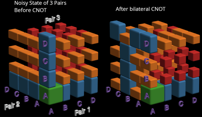
On the left we have a visualization of a noisy Werner state ρ₀ ⊗ ρ₀ ⊗ ρ₀ (as defined in the main text). Each colored solid corresponds to the probability weight of a given pure basis state, as labeled in purple, with larger solids corresponding to a higher probability. We have 3 axes, one for each subsystem. The green solid corresponds to the “good” state (leftvert Arightrangle otimes leftvert Arightrangle otimes leftvert Arightrangle), the one of highest probability. Blue solids correspond to basis states in which one of the 3 pairs has experienced an error. For orange (and red) we have two (or all three) of the pairs having experienced an error. On the right, we have the resulting state after Alice and Bob perform bilateral CNOT gates on pairs 2 and 3. This interpretation of bilateral gates in terms of a permutation of the Bell basis permits much faster simulation of entanglement distillation circuits, as discussed in section II A.

Full size image

There are two steps where we model error: in the generation of a raw Bell pair and in 2-qubit gates and measurements. We can represent any set of Bell pairs with a density matrix diagonal in the Bell basis, however for initial raw pairs we typically pick the Werner state ({rho }_{0}={F}_{{rm{in}}}leftvert Arightrangle leftlangle Arightvert +frac{1-{F}_{{rm{in}}}}{3}(leftvert Brightrangle leftlangle Brightvert +leftvert Crightrangle leftlangle Crightvert +leftvert Drightrangle leftlangle Drightvert )), where the different Bell states are:

F_in is the fidelity of a raw Bell pair while 1−F_in can be thought of as the overall error or infidelity.

For 2-qubit gates, we assume the gate acts correctly with probability p₂ and completely depolarizes both pairs involved with probability 1−p₂. However, if more information about the types of biased errors on any particular hardware system is known, our framework can be used to model those errors instead (as long as they can be represented by a Pauli channel). For most of the numerical experiments in this text, following typical current hardware parameters, the error rate of raw Bell pairs is on the order of 10%, the error rate of 2-qubit gates is on the order of 1%, and we do not consider 1-qubit gates since their error rates are much smaller.

For measurement errors, we assume that with probability η the correct results of the projection are returned, with probability 1−η the incorrect result is returned. When not specified, we assume η = p₂. The allowed measurements are coincidences in the X and Z Pauli eigenbases and anti-coincidence in the Y eigenbasis, which each “select” (i.e., report a “coincidence”) for the state (leftvert Arightrangle) and for one other Bell state. In other words, when these measurements fail (differing results for coincidence and same results for anti-coincidence), Alice and Bob have detected an error in one of our Bell pairs so they restart the procedure.

Lastly, before exploring the zoo of highly optimized purification circuits we have discovered, we need to discuss a variety of optimization targets and cost functions available to us. As discussed later in this text, this choice can be crucial for the overall performance of a quantum network. For the majority of the presented results we consider a quantity denoted F_out which we call “average marginal fidelity”. The states we consider have diagonal density matrices in the multi-pair Bell basis, and as such can be interpreted as a discrete probability distribution over multiple variables—each variable corresponds to one of the Bell pairs and each of the discrete possibilities is whether we have an A, B, C, or D state. The marginal probability to have the ith pair in state A, averaged over the indices i corresponding to purified pairs is F_out. In a typical “physical” notation that is

where k is the number of purified pairs, ρ is the final multi-pair density matrix, and ptrace_S is the partial trace over all subsystems not in the set S. We stress that directly computing F_out in our simulations is more straightforward than the expression given above implies, thanks to the data structures we use, as discussed later in this text.

In a few specific contexts, we also consider the more typical^{18,19,20,22,29,30} figure of merit F_A corresponding to all purified Bell pairs being in state A:

We show that this very common choice of figure of merit can be detrimental, and provide better alternatives to it (e.g., F_L F_out defined below).

Another metric we consider is success probability. This is the probability of the circuit having a successful run, which corresponds to Alice and Bob never restarting their procedure based on their measurement results. This is a worst-case bound, as in many cases it is feasible for Alice and Bob to restart only a small part of their circuit without starting from scratch.

All of these figures of merit and more are easily evaluated with our simulation algorithm and as we will see in the following discussion have differing degrees of practicality. F_A is a common choice because of its simple interpretation (probability of having no error in any of the Bell pairs), but later on we see that full-stack alternatives (modeling the performance of the entire application running on top of the purification) can be much better. It can be potentially important to also take into account rates and probabilities of success, for which various yields can be defined²⁶. In³¹ a variety of upper limits on some of these figures of merit are discussed.

Optimized purification circuits

We explored several situations where our optimization approach, enabled by the new method for fast simulations, provides state-of-the-art n-to-k purification circuits. First, before studying specific important cases, we will present a survey over a wide range of circuit parameters, showcasing both the ease with which our technique can be employed and a number of important trade-offs in the design of purification circuits. For illustration purposes, Fig. 2 presents a typical discovered (optimized) purification circuit.

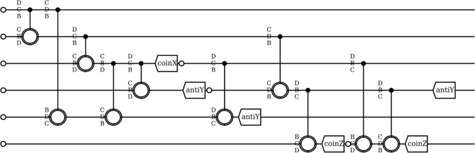
This circuit produces k = 3 purified Bell pairs using n = 9 raw Bell pairs in a circuit of width r limited to no more than r = 6 (i.e., maximum number of qubits that can be stored at the same time). The 9 small open circles (seen at the beginning of the circuit and after intermediary measurements) signify the generation of a raw Bell pair in that register. Note that we are only showing Alice’s circuit and that Bob performs the same operations on his circuit. CNOTs are preceded by a permutation in the Bell basis and these are together shown as open circles with the permutation written out to the left (the notation and choices of good permutations is dicussed in Section II C). The measurements are labeled with whether they are coincidence or anti-coincidence and in which Pauli eigenbasis they are performed.

Full size image

For an initial parameter-sweep population study, we consider n-to-k purification circuits, on registers of varying size (the number of qubits that can be stored simultaneously, i.e., the maximum width of the purification circuits, denoted by r). The consideration of register size limitations is quite crucial, as many of the otherwise-optimal well-known recursive purification circuits from the literature^18,19,20,21 are impossible to implement on small-size registers. We denote n the number of initial raw pairs, k the number of preserved pairs, and r the size of the register. With register reuse r < n is permitted, but naturally we need k < r for any purification to be possible. In this parameter sweep we consider r up to 8, k up to 7, and we do not bound n. The noise of the two-qubit gates is also taken into account: a crucial limiting factor very rarely considered in most literature on the topic (see refs. ^22,23,25,26 for some of the few works dealing with gate noise in purification circuits). The resulting circuits are summarized in Fig. 3. One of the more important features that can be observed is the need for a register wide enough to contain more than two sacrificial pairs—otherwise the error detection capabilities of the circuit are restricted as previously observed in refs. ^22,26. There is a trade-off between the probability of success and fidelity, which is also dependent on the number of sacrificial pairs (more thoroughly investigated in Fig. 4). That figure also shows an asymptote for the achievable fidelity, present due to gate noise (in the absence of scalable large registers permitting error-correcting gates).

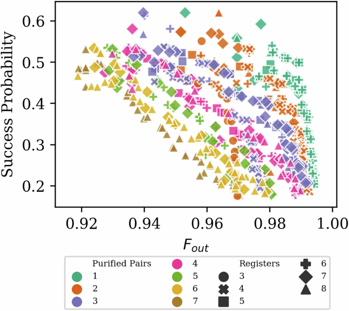
The horizontal axis is F_out – the fidelity of the purified pairs, the vertical axis is how likely the procedure is to succeed, the colors show k – how many pairs the circuits purify to, and the shapes show r – the width of the circuit, i.e., the minimal size quantum memory capable of storing the necessary qubits. The optimizations were done at F_in = 0.9, p₂ = 0.99 without restricting the number of raw Bell pairs (n) or circuit length (visualized in the following figures). The most appropriate circuit to choose from this population would depend on hardware constraints and application-level goals as described in the main text. Importantly, the optimization can easily be redone to fine-tune the circuits for particular hardware subject to arbitrary Pauli noise. Some general trends we see are: increasing the number of preserved purified pairs leads to lower fidelity, while more sacrificed pairs lead to higher fidelity; increased fidelity comes with decreased success probability; increasing register width tends to increase fidelity but the increase gets saturated quickly at r = n + 2^22,26 – easily seen in the k = 2 and k = 3 cases at various r and in the r = 7 and r = 8 cases at various k. These trends are explored in more detail in Fig. 4 where the dependence on n is elucidated as well. We do not consider cases where k and r are very close as there are no interesting circuits in that regime, due to the impossibility of simultaneous multi-pair sacrifices.

Full size image

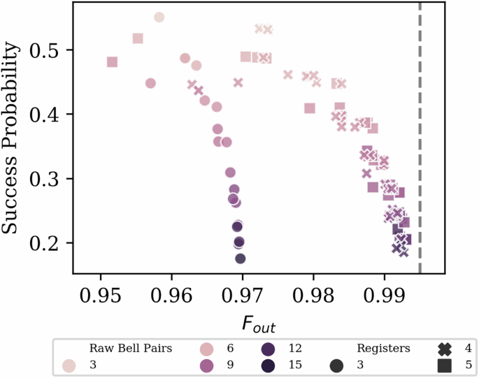
Each data point is an n-to-2 circuit evaluated at F_in = 0.9, p₂ = 0.99. Axes as in Fig. 3, color indicates n the number of raw Bell pairs used, shape indicates r the size of the quantum memories. We see that increasing the number of raw pairs sacrificed corresponds to higher F_out since we can perform more rounds of error detection, which however leads to decreased single-shot success probability. There is a jump in F_out as the register width grows from three to four since four registers are the minimum needed to perform “double selection”²². Once this minimum is met, the circuits approach the upper bound on fidelity, shown as a vertical dashed line which is set by the error of the last operations performed²⁶.

Full size image

With the faster simulation methods we have developed, such a population study can be performed in minutes on commodity classical hardware. For pedagogical purposes, we picked fairly generic parameters, but any hardware developer can easily redo the simulations, taking into account biased noise typical for their platform, memory errors, or finite wait times between raw pair generation. This co-design process provides significant gains in performance, compared to applying simple generic purification circuits as seen from comparisons in the following paragraphs.

Moreover, colleagues studying methods for an exhaustive enumeration of possible purification circuits have graciously provided comparisons between our optimization techniques and a few “known best circuits in the absence of gate noise”³⁰, giving additional proof of the high performance of our circuits. Below we continue with comparisons to typical small purification circuits.

Comparison to other methods

There are very few non-asymptotic designs for n-to-k circuits^{22,23,24,25,26}, virtually none that are designed with gate (a.k.a. “operational”) noise constraints in mind. Even “information-theoretically perfect” methods like the hashing protocol³⁴ fall short when applied to finite circuits or when gate noise is present. Below we compare our optimized circuits to straightforward concatenations of known protocols and truncated versions of the otherwise asymptotic “perfect” hashing protocol, showing we significantly outperform both approaches.

Consider the well-known single- and double-selection^22,23 circuits. We compare against manually generated circuits built from these sub-circuits in Figs. 5 and 6. The increase in performance of our optimized circuits comes from being able to entangle more Bell pairs before measuring and detecting errors, which we are confined to in a modular setting. For the same reason, our technique can provide the same final fidelity at much lower hardware requirements.

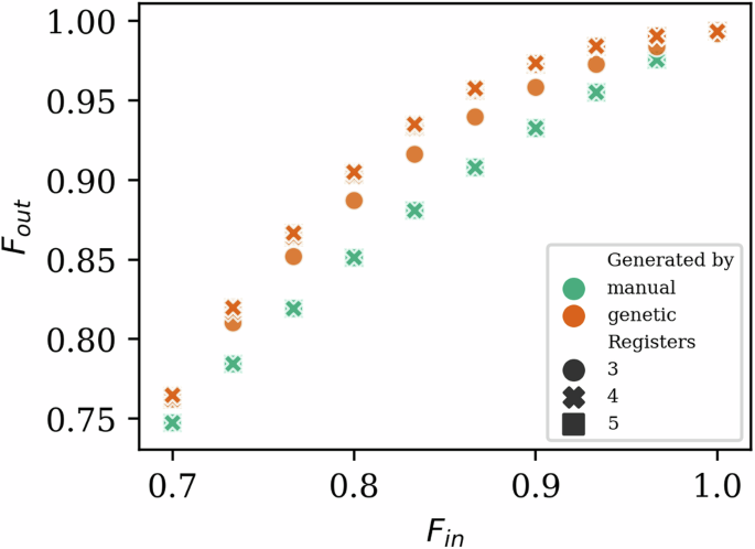
The plot is F_in versus F_out, the colors represent whether the circuit is manually created from standard sub-circuits found in the literature^18,19,20,22 or generated by our optimizer, shape indicates r the size of the quantum memories. Examples of these circuits can be found in Fig. 6. Our optimized circuits outperform circuits built from single and double selections sub-circuits in a wide range of raw Bell pair fidelities and can have smaller register widths. The circuits are evaluated at p₂ = 0.99.

Full size image

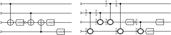
The circuit on the left is manually created, with a single selection circuit followed by the most appropriate double selection. On the right is an example of a circuit found by the optimizer.

Full size image

On the other end of the spectrum, consider the hashing protocol which early on was designed to saturate information-theory bounds about purification performance (assuming asymptotically many pairs in unbounded register with perfect gates). We next evaluate our methods against the hashing protocol when it is truncated to fit on finite hardware. The truncated hashing protocol works best when purifying to and from powers of two Bell pairs, so for that reason, we show 8-to-2 circuits in Fig. 7. Similarly to the previous comparison, we significantly outperform hashing, especially with noisy gates.

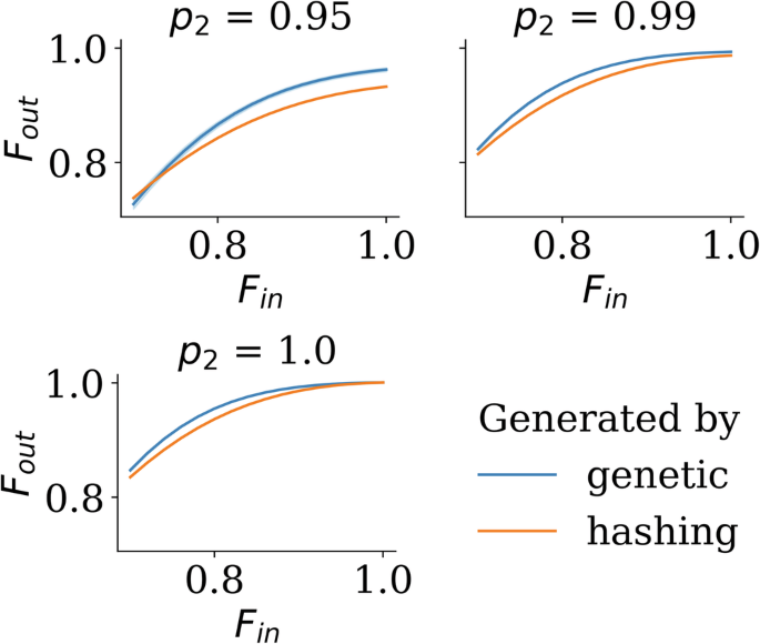
The plot is F_in versus F_out, the blue is our circuits while the orange is the truncated hashing protocol circuit, and we have three sub-graphs at different gate fidelities. The optimized circuits outperform the truncated hashing protocol at various hardware parameters after being optimized for F_in = 0.9, p₂ = 0.99, chiefly because (1) the hashing protocol is optimal only in the asymptotic limit of infinitely large registers and (2) the hashing protocol’s optimality proof assumes its is running on perfect hardware, while we optimize our protocols in the presence of hardware noise.

Full size image

Both of these alternative methods we compare against are in settings they are not optimized for, but nonetheless, they are the only techniques otherwise available. It is worth noting that there is a correspondence between n-to-k purification protocols and [[n, k]] error correcting codes, but similarly to the troubles with the hashing protocol, studying that correspondence does not take into account the finite size of available registers, the gate noise in those registers, and the exact layout of the gates in such a circuit.

It is worth reiterating that one of the bigger advantages opened by our method of “faster simulation enabling bespoke optimization” is that we can produce circuits specifically tuned to a particular error model. This advantage is particularly evident when we compare to exhaustive circuit enumeration techniques (which are currently available only for simpler noiseless circuits) E.g. in recent work³⁰ (Fig. 14) Goodenough shows that their exhaustive enumeration of circuits provides better “noiseless” circuits, but these circuits perform worse than what we can generate when accounting for hardware noise.

The optimized purification circuits we find do not have specific interpretable features—a result typical for black-box optimizations over detailed hardware models. If such interpretable features were discovered, they would lead to an even faster simulation and optimization algorithm than the new simulation algorithm we discovered. Through Figs. 1–4 we describe some trends with respect to hardware parameters. One overall feature that is worthwhile to call out is that our circuits do not have subcircuits that can be easily factored out like in a typical recursive or hashing purification protocol. Rather, our circuits perform large multi-qubit permutations (whichever ends up optimal for the given noise bias). This feature can be recognized in early attempts of gate-noise-aware purification like double selection²².

More generally, optimization methods like ours permit co-design of both the abstract purification protocol and the circuit compilation itself, which is extremely valuable if the hardware has some limited qubit-connectivity topology. E.g. if our qubits permit only nearest-neighbor gates, it is not enough to know the best purification protocol, but rather the best protocol given the limited qubit-connectivity. Instead of solving the purification protocol design and the circuit compilation problem separately, optimizers like ours solve both problems together, providing for much higher performance compared to concatenating two independent solutions (e.g., ref. ³⁰).

Application to error correction and teleportation

Here we pursue a more sophisticated example of such co-design, where we do not simply maximize the performance of a single purification circuit, but rather the performance of the entire application stack built on top of the purification circuit. Consider the use of Bell pairs in teleportation of error-protected states for instance. Going beyond 1st generation quantum repeaters³⁵, teleportation and error correction become important additions on top of the entanglement distillation and swaps, and this is a natural application for our purification circuits. In particular, we investigate the following protocol stack running on two nodes between which we can establish noisy entanglement:

• Purification of n raw Bell pairs into k higher quality pairs.

• Teleportation of (fewer than k) logical qubit(s) encoded in the k physical qubits from one node to the other.

• Error correction on the logical qubit(s) after teleportation.

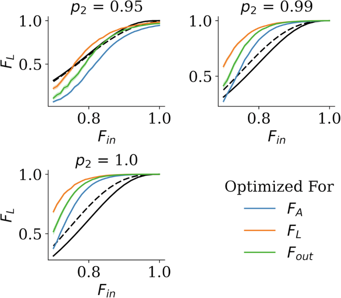
We can then determine the quality of the procedure by how likely it is that the logical qubit is in its original state after teleportation and error correction. This overall probability we will call the logical fidelity F_L. Note that in calculating F_L, we assume the local gates for the error correction procedures are noiseless, in order to focus on the purification step (but including noisy gates for the error correction would be straightforward). We show results when using the 5-qubit^34,36 and a [[11, 1, 5]] error correction codes (the smallest to correct for two-qubit errors³⁷), but the technique is generally applicable to any stabilizer code.

The overall theme behind the results is that by doing full-stack optimization instead of optimizing only for entanglement purification fidelity, we consistently obtain circuits with significantly better performance for the two codes we have considered as seen in Figs. 8 and 9. The exact circuits are specific for the network error model, gate error rate, error correction code, and other constraints, thus we do not plot them here, however, they can be seen in the archived software repository or regenerated within minutes thanks to the provided software (while also being optimized for the particular hardware parameters that matter to the downstream user).

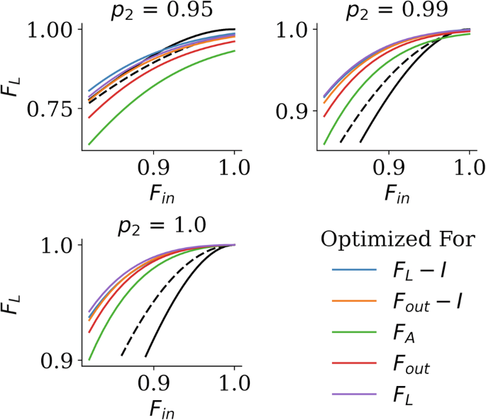
The plot is F_in versus the fidelity of the logical teleported qubit after error correction F_L, while the colors signify what the circuits were optimized for. The solid black line shows the performance of using unpurified pairs for teleportation, and the dashed black line shows the performance when using the typical 2-to-1 single selection purification protocol (equivalent to truncating the hashing protocol). Surprisingly, we see that optimizing for purification fidelity (F_A or F_out) leads to significantly lower overall performance. As discussed in the main text, this is due to not constraining the long tail of correlated multi-qubit errors. All optimizations were done at raw Bell fidelity F_in = 0.9 and local gate fidelity p₂ = 0.99, but we plot the performance at various p₂. If the p₂ value is known for a given hardware, the circuit should be optimized for that value. Cost functions that include a “mutual information” term I are included here and discussed further in the appendix, were we also further explore various circuit parameters, like circuit length and width.

Full size image

The plot is F_in versus F_L, the colors signify what the circuits were optimized for, the solid black line shows the performance of using unpurified pairs for teleportation, and the dashed black line shows the performance when using the 2 to 1 single selection protocol to purify pairs. We see similar trends as we saw with the 5-qubit code in Fig. 8, which shows how our method can scale for larger codes and code distances. These circuits use 14 registers and are evaluated with 100,000 Monte Carlo runs.

Full size image

We explored three main cost functions in our optimizer. The first is F_out, which is the average marginal fidelity of each of the purified pairs (the metric we use throughout most of the paper as a proxy for quality of purification). The second is F_A, which is the probability that all the purified pairs are to be Bell pair A, i.e., the overlap of the final purified state with the state ({leftvert Arightrangle }^{otimes k}) – this is another very common measure of quality of purification. The third is F_L, which is the probability of no logical error after teleportation (i.e., the probability for fewer than d/2 errors in the purification protocol, where d is the code distance). This third cost function is equivalent to the fidelity of the teleported logical qubit.

The surprising result we observe is that optimizing for high-quality purification does not result in high-quality overall protocol performance, underscoring the importance of co-design. The intuitive reason behind this effect is that a cost function that focuses on high-quality purification does not constrain the long tail of the probability distribution over possible errors, which is crucial to the performance of an error-correcting code. I.e., F_A and to a lesser extent F_out penalize low-weight and high-weight errors equally. Conversely, one can interpret the F_L cost function as forbidding multi-qubit errors while permitting correctable errors, i.e., errors with a weight smaller than d/2 where d is the distance of the code layered on top of the purification. Other measures of error correlation were also considered as cost functions and discussed in the appendix.

Faster simulation of entanglement circuits

We now introduce the faster simulation algorithm that made much of the optimization work possible. Typical entanglement purification circuits are Clifford circuits used on stabilizer states, for which there are known polynomial algorithms^38,39. The well-known Stabilizer tableaux representation typically takes ({mathcal{O}}({N}^{2})) space complexity, where N is the number of qubits. Applying a single gate takes ({mathcal{O}}(N)) time, and a measurement takes ({mathcal{O}}({N}^{2})). The graph state formalism is even faster (for sparse tableaux), with ({mathcal{O}}(Nlog N)) space complexity⁴⁰.

In order to design a more effective algorithm to simulate purification circuits, we propose a more efficient representation of Bell states and purification circuits. We limit ourselves only to multi-pair mixed state entanglement purification. We consider states whose density matrix is diagonal in the Bell basis {A, B, C, D}^⊗n (n is the number of Bell pairs).

A crucial restriction in our representation is based on the realization that a purification circuit consists of two simple stages: bi-local unitary gates that act as permutations in the Bell basis and a coincidence measurement that acts as post-selection, zeroing out exactly half of the components of the diagonal of the density matrix. The group structure of such permutation circuits has been studied extensively^29,41. A good purification circuit is one for which the Bell basis permutation that it performs is the one that maximizes the probability to be left with the desired final state. Insight from that group structure has been used to enumerate good purification circuits²⁹.

These restrictions are not limiting us when studying entanglement purification: noisy entangled states with a density matrix non-diagonal in the Bell basis can easily be converted into diagonal ones through a modified twirling operation without changing the output fidelity of the purification circuits (for all fidelity measures presented in this work). Also, Bell-diagonal states naturally arise with realistic noise models such as dephasing and depolarizing.

More efficient state representation

Each gate in the purification circuit, and thus the whole circuit, can be thought of as a permutation of Bell basis, and measurement can be thought of as cutting the space of possibilities in two. Such operations preserve the block-diagonal form of the tableaux and only change the phases column. Thus we only need to track these phases. Consider the following state

where the omitted off-diagonal entries are identities II.

We track only phases of this state, where + is represented by 1 and − by 0. Then, the above state can be represented by 110010. The new representation will only need 2n bits to represent a state of n Bell pairs. We call this new representation a diagonal representation. The space complexities of diagonal, state-vector (a.k.a ket or wavefunction), and tableaux representations are summarized in Table 1. Note that state vector representation is fully general, while tableaux represent a subset of possible states, and the diagonal representation covers an even smaller subset, thus trading off generality for efficiency.

A bi-local gate from a purification circuit is now simply a permutation over the set of integers (represented by the aforementioned bitstrings). As we discuss below, not all such permutations are valid gates.

Note that noisy dynamics still require a Monte Carlo simulation, but unlike the Clifford approach, we only need ({mathcal{O}}(1)) complexity per gate instead of ({mathcal{O}}(N)). This improvement in efficiency can be thought of as hard-coding the sparse nature of the tableau. The new representation is able to model any Pauli noise.

Our diagonal representation also has a similar performance to the “Pauli frames” approach, but our diagonal representation does not require the simulation of reference frames. Moreover, the more constrained representation of permitted Bell-purifying gates was crucial for the efficient search for good purification circuits—a feature lacking in Pauli frame simulations.

“Bell Preserving” gates

Above we discussed the state representation. Here we follow with a discussion of the dynamics of these states. We consider only operations that preserve the Bell-diagonal nature of our states. Let us call the set of such gates “Bell Permuting” or “Bell Preserving” (BP). Let us denote the set of BP gates on n Bell-pairs as ({{mathcal{B}}}_{n}). It has been known for a while what that group is, and it even has its own (as efficient as Clifford) implementations based on symplectic matrices⁴¹. Our work can be restated as the simple realization that these operations have much more compact representation as (canonically enumerated) permutations. We further describe a simple “fixed length” representation (and enumeration) of these BP gates, particularly convenient for software simulations or random sampling.

First note that BP gates are a subset of Clifford gates. Denote all Clifford gates on N qubits as ({{mathcal{C}}}_{N}) (for which we also can derive (| {{mathcal{C}}}_{N}| =2({4}^{N}-1){4}^{N}| {{mathcal{C}}}_{N-1}|)). We also use ({{mathcal{C}}}_{N}^{* }) to denote Clifford gates that do not specify phases, i.e., ({{mathcal{C}}}_{N}^{* }={{mathcal{C}}}_{N}/{{mathcal{P}}}_{N}) where ({{mathcal{P}}}_{N}={{sigma }_{1}otimes cdots otimes {sigma }_{N}| {sigma }_{i}in {I,X,Y,Z}}). Thus we have ({{mathcal{C}}}_{N}=left{Ccdot P,| ,Pin {{mathcal{P}}}_{N},Cin {{mathcal{C}}}_{N}^{* }right}) and (| {{mathcal{C}}}_{N}^{* }| =frac{1}{{4}^{N}}| {{mathcal{C}}}_{N}|).

Observe that Bell Preserving gates on n Bell pairs are always bi-local Clifford gates. Similarly to the introduction of Clifford gates up-to-a-phase, we introduce

for which there is a known identification⁴¹

where Sp denotes the symplectic group.

We focus on the group ({{mathcal{B}}}_{2}) as that is the set of operations typically available in a quantum computer (i.e., two-qubit gates). We can observe that ({underbrace{g}_{{Alice}}otimes underbrace{g}_{{Bob}}| ,gin {{mathcal{C}}}_{2}^{* }}subset {{mathcal{B}}}_{2}^{* }) and that they are of equal size. This simple counting argument gives us

The n > 2 case is briefly discussed in the appendix, but the counting argument fails for it and there is no such simple representation.

Lastly, to complete the enumeration, and to provide efficient sampling, we need a convenient way to represent ({{mathcal{C}}}_{2}^{* }). Figure 10 depicts a useful decomposition in a set of cosets (Q={{mathcal{C}}}_{2}^{* }/({{mathcal{C}}}_{1}^{* }otimes {{mathcal{C}}}_{1}^{* })), which provides 20 distinct “inherently two-qubit” gates (i.e., ∣Q∣ = 20). This coset decomposition lets us separate the “inherently two-qubit” part of the circuit from the single-qubit dynamics. However, there is no one unique way to pick an element from each coset, so we are left with some arbitrariness in the choice of the 20 gates. We pick one particular set for our software implementation, such that gates like SWAP and CNOT are contained in it for convenience, and with slight abuse of notation we also denote it Q.

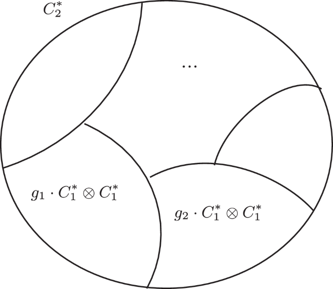
All “phaseless” two-qubit Clifford gates can be decomposed in the product of one of 20 “inherently two-qubit” gates, and two single-qubit phaseless Clifford gates (six options for each). This exposes the coset structure of ({{mathcal{C}}}_{2}).

Full size image

Putting all this together, a Bell-preserving ({{mathcal{B}}}_{2}) gate can be written as

where (pin {{mathcal{P}}}_{2}) and (gin {{mathcal{C}}}_{2}^{* }) can be written as

where (hin {{mathcal{C}}}_{1}^{* }) and (fin {{mathcal{C}}}_{1}^{* }) and g₀ ∈ Q. Thus, a general gate in ({{mathcal{B}}}_{2}) can be represented as in Fig. 11, where ({p}_{1},{p}_{2}in {{mathcal{P}}}_{1}) Pauli gates (4 possibilities each), (h,fin {{mathcal{C}}}_{1}^{* }) single-qubit Cliffords (6 possibilities each), and ({g}_{0}in Q={{mathcal{C}}}_{2}^{* }/({{mathcal{C}}}_{1}^{* }otimes {{mathcal{C}}}_{1}^{* })) “inherently multiqubit” gates (20 possibilities). Thus, we have

different 2-pairs BP gates. The coset decomposition is partially discussed in refs. ^29,30,42.

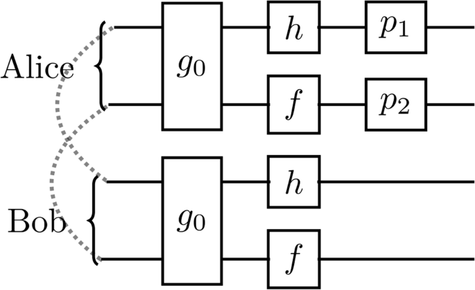
The dashed lines represent the two initial Bell pairs while the brackets denote which node (Alice or Bob) stores the qubits. Except for ({p}_{1},{p}_{2}in {{mathcal{P}}}_{1}) Pauli gates (4 possibilities each), the circuit is symmetric between Alice and Bob. Namely, they both perform (h,fin {{mathcal{C}}}_{1}^{* }) single-qubit Cliffords (6 possibilities each), and ({g}_{0}in Q={{mathcal{C}}}_{2}^{* }/({{mathcal{C}}}_{1}^{* }otimes {{mathcal{C}}}_{1}^{* })) “inherently multiqubit” gates (20 possibilities).

Full size image

Lastly, it is useful to restrict oneself to an even smaller set of gates, namely gates that act as the identity when restricted to “good” entangled states, i.e., permutations for which (leftvert AArightrangle mapsto leftvert AArightrangle). These “good” gates are a subset of the aforementioned Bell permuting gates and we have provided an interface for it in our implementation of the simulator. This leads to a fairly small set of necessary gates: CNOT as the only two-qubit gate, and single-qubit gates that simply permute among the B, C, and D states. In the circuits we have plotted we denote the single-qubit gate permutations as follows: a gate that permutes BCD to DCB is simply denoted by the DCB string. Our simulation algorithm can easily be expanded to multi-qubit gates and even to the simulation of purification of graph states, however this was not necessary for the optimization runs we showcase.

The gate representation we introduced in this section has numerous benefits. First of all, while there are many other ways to represent a permutation of a set, the representation we introduce ensures that we work only with valid bi-local gates of the Bell basis that can actually be realized by Alice and Bob—the valid permutations are a subset of all possible permutations. Moreover, our representation makes it trivial and efficient to pick a permitted operation at random, uniformly over the set of all permitted permutations. Lastly, the representation is of fixed size (unlike many other data structures representing permutations), namely a tuple of five bounded integers. This regularity provides for much more efficient (contiguous) storage of circuits as arrays of gates in computer memory, which is crucial for cache coherence and high-speed CPU performance.

Software implementation

One immediate application of the above result is a more efficient implementation of a simulator for purification circuits. Specifically, instead of working with stabilizer tableaux and arbitrary bi-local four-qubit gates, we can decompose each of the BP gates into one of the 20 two-qubit gates (Q), two of the 6 one-qubit phase-less gates (({C}_{1}^{* })), and two Pauli gates. Internally, each of these subgroups of gates is represented as a subgroup of permutations over integers and the bitstring representation of the integers coincides with a particular set of Bell pairs as discussed above. Thus any bi-lateral gate can be fully defined by 5 indices. With the diagonal state representation, the application of any of the 11520 BP gates takes ({mathcal{O}}(1)) steps simply a mapping from one bitstring (a 2-bit or 4-bit integer) to another bitstring.

Using diagonal state representation and Bell-Preserving gates, we can significantly improve the performance of purification circuit optimization since the gate representation is extremely compact and of fixed length and it takes constant time to apply. To model noisy systems we can either employ Monte Carlo simulations giving us numeric result, or do a perturbative expansion over the most probable trajectories giving us both a symbolic and numeric results.

The BP representation is implemented in the Julia language as the BPGate.jl package. We compare the performance against a thoroughly optimized tableaux simulator (QuantumClifford.jl) and wavefunction simulator (QuantumOptics.jl, including both dense and sparse matrix representations of operators). In Fig. 12, we plot the run time of applying a bilateral CNOT gate to two randomly chosen pairs of Bell pairs in the network against the number of Bell pairs in the entanglement network. The run time of BPGates is independent of the number of Bell pairs in the network (({mathcal{O}}(1))), which improves from the linear runtime of the Clifford representation and exponential runtime using the matrix representation.

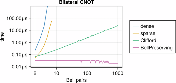
As expected, a full-state vector simulation is exponentially expensive, independently of whether the operator is represented as a sparse or a dense matrix. Much more interesting is the comparison between a typical Clifford circuit simulation (here using the highly optimized QuantumClifford.jl implementation) and our new BPGates.jl implementation based on the methods described in this paper. Additionally, BPGates.jl provides for very compact parameterization of all possible purification circuit gates, lending itself to use in circuit optimizers.

Full size image

Above we have discussed the implementation of ({{mathcal{B}}}_{2}), but a purification circuit may involve permutation of more than 2 Bell pairs. Naturally, any such larger circuit would need to be decomposed in two-qubit gates to be executed on a quantum device. We have also restricted ourselves only to bi-partite entanglement, but similar “block-diagonal tableaux” and “base-preserving gate” formalism exist for the purification of any multipartite entangled stabilizer state.

This paper introduces three important new directions to the theory and practice of quantum networking. The new entanglement purification simulation algorithm we introduce has much lower complexity than the alternatives. Moreover, it provides for very natural parameterization of permitted gates in a purification circuit. Of course, with higher performance, comes specialization, thus the algorithm applies only to distillation circuits.

This algorithm enabled circuit optimization at a previously impossible scale. Not only was the cost of simulating a single state too high, but due to the unstructured nature of the search space a vast array of simulations need to be executed. This is now practical and any new search method can benefit from the improvements we have enabled. The optimized circuits we can now generate are superior to anything else currently available for noisy hardware^{22,23,24,25,26} and can be fine-tuned to the particular noise model of the hardware that will be executing them. The only prerequisite on the experimental side is to perform detailed tomography for the (potentially biased or correlated) error model of the hardware so that the circuit simulator and optimizer have a correct cost function.

Lastly, we demonstrate that optimizing common choices of figures of merit can be misguided and even detrimental depending on the network application. In the typically studied asymptotic case, the difference is insignificant, but when one considers the constraints of a finite-size quantum register, it becomes important to employ a specialized figure of merit. For instance, we show that if the entanglement purification is used as the physical layer under the teleportation of logical qubits, then the typical definition of fidelity (denoted F_A here) is the one that leads to the worst possible performance. This happens because F_A does not distinguish between low-weight and high-weight correlated errors, while this distinction is crucial to the performance of the error correction code at the next layer of the technology stack.

Numerous further steps can be taken to improve these results. Our superior simulation algorithm can be repurposed for the modeling of the purification of arbitrary graph states. That would require generating a new set of “good” gates (and corresponding permutations) for each class of graph states. Thankfully this process can in principle be automated in software. But even restricting ourselves to cases of Bell pair purification there is much more that can be done on the engineering side, including more detailed parameter sweeps of best circuits for various types of hardware, and for various applications (similarly to the entanglement teleportation example we gave in this work). In the optimizations we performed we did not model classical communication delays or the rate-fidelity tradeoffs in generating raw Bell pairs, however, there is no technical difficulty in including these effects, and they are to be added to our open-source simulator in the near future. We only focused on the entanglement distillation task in this work, but our efficient modeling algorithm can be trivially extended to model swapping as well, for studies involving long repeater chains. Lastly, there is a rich design space to be explored that studies how to best create high-fidelity multi-party entangled states—in what order should we nest Bell state generation, Bell state purification, entanglement swapping, merging of Bell pairs into larger graph states, and graph state purification itself. Many of these tasks are now much easier to model thanks to our work, but there is still much more to explore.

When considering future directions, it is worthwhile to note that in this work our chief advantage was making the “inner loop” of the optimization algorithm much faster, i.e., we simulate the system-to-be-optimized much faster than previously possible, but we have not improved upon the state of the art in the optimization algorithm itself. We want to design our circuits for realistic hardware noise models, which makes the problem not amenable to structured optimization approaches (as the elegant analytical description³⁰ available for noiseless circuits is now lost). However, we envision future projects to significantly improve the “outer loop”, moving away from our unstructured optimization heuristics to a more principled approach. E.g., we are working on a computer algebra system (as part of the already public QuantumClifford.jl package) that would let us do “semi-symbolic” perturbation expansions of the final figure of merit (e.g., fidelity or probability of success) with respect to various noise or circuit parameters, potentially enabling better optimization techniques exploiting this symbolic information.