Forest fires under the lens: needleleaf index – a novel tool for satellite image analysis
Introduction
The boreal forest, referred to in North America as Taiga, is the Earth’s second-largest land biome and is dominated by coniferous forests, including spruce, fir, pine, and larch forests. Boreal forests are of global importance because of their significant carbon stocks, freshwater resources, biodiversity, and use for lumber and other wood products6,7,8,9,10. The global forest area in 2020 was approximately 40.58 million km2, which is 31% of the total land area, while 10.95 million km2 (27%) of the world’s forests are in boreal domains11. The total carbon storage values of boreal forests are approximately 367.3–1715.8 Pg7. Boreal forests are expected to experience a substantially more significant increase in warming than any other forest ecosystem12.
Boreal forests face many challenges, including climate change, wood production, and drought12,13,14. Climate change significantly affects different species in boreal forests and is expected to affect forest composition in the future15. Climate change, wildfires, and lumber harvesting reduce tree cover along southern biome boundaries16. In Canadian boreal forests, rising temperatures along with decreased precipitation are likely to contribute to an increase in the frequency of extreme weather events, fires, and a dry climate14,17,18. It appears that boreal forests are shifting from being carbon sinks to carbon sources, particularly in western Canada, where boreal forests may release more carbon dioxide into the atmosphere than absorb it7,12,19. Additionally, changes in the expansion of boreal forests are expected to result in changes in albedo. The cooling impact of albedo can increase when a boreal forest area is reduced or when coniferous species change to broadleaf tree species16.
Remote sensing (RS) is a valuable tool for studying and monitoring boreal forests because it provides detailed information about their characteristics and changes over time20,21,22. Considering the global coverage, spatial resolution (30 m), and long-term observations (more than 50 years)23, Landsat Earth observation satellite data are the best source of information for investigating past forest cover conditions24,25. Furthermore, the advantages of Landsat RS data, including free access and repeated observations, make land cover monitoring more accessible and more accurate23,26. RS satellites provide long-term images to study land cover dynamics and are particularly efficient for detecting changes in vegetation cover27,28,29. Multiple RS indices have been developed to investigate different land cover types, specifically forests, via spectral bands30,31,32,33. Identifying changes in vegetation indices could be challenging due to the difficulty distinguishing between canopy forests and other vegetation types16. Vegetation indices such as the normalized difference vegetation index (NDVI)30, soil-adjusted vegetation index (SAVI)31, and enhanced vegetation index (EVI)32 enhance the vegetation signal by combining different spectral bands and highlighting plant properties. During the growing season, NDVI saturation occurs, but the SAVI and EVI perform better than the NDVI in highly vegetated areas and are less prone to saturation34,35. However, these known indices are not specialized for coniferous forest detection and cannot be used to distinguish coniferous forests from other vegetation cover types alone. The forest index33 (FI) is another advanced spectral index used to differentiate between forests and other land cover types. It is calculated via the green, red, and near-infrared bands. The FI can be used to classify images into forest and non-forest areas; however, this index is not optimized to detect coniferous forests because it requires green and red bands and coniferous forests exhibit the same spectral reflectance as other vegetation covers4 in these bands. Hence, there is a need for a spectral index that can accurately detect coniferous forests.
Comprehensive and precise coniferous forest area (CFA) estimations are necessary to perceive and predict spatiotemporal changes in forest capacity; currently, datasets for conifers, which are the major staple of the Canadian boreal forest, are inadequate. Boreal coniferous forests in North America are experiencing a significant decline, according to global forest loss mapping conducted between 2000 and 2012 via Landsat data36. Several scholars have studied North American boreal forests via Landsat imagery; these studies have investigated boreal forest cover loss16, mapping, and impacts on wildfires37,38, boreal forest recovery rates22, biomass estimation39, and mapping disturbances in boreal ecosystems40.
One of the drawbacks of RS is its computational complexity when large areas are mapped. However, the Google Earth Engine (GEE) geospatial processing platform effectively overcomes this difficulty. Cloud-based platforms, such as GEE, are capable of quick and easy sampling, analysis, and monitoring of planetary-scale geospatial data through parallel processing41,42. GEE has free access to massive volumes of satellite dataset archives and algorithms for processing remotely sensed imagery and was developed by Google in 2010. In this study, all the Landsat data processing was managed via cloud computing technology in the GEE environment. Another major limitation of optical remote sensing is the existence of cloud cover in the image scenes43. The amount of cloud cover changes daily, annually, and geographically44. Cloud cover poses a severe challenge to Landsat, which requires 16 days to acquire a new image based on its revisit time. To address this issue, it is better to utilize summer image acquisitions, which result in less cloud coverage. Additionally, incorporating cloud masking techniques and using data from multiple sensors can further mitigate the impact of cloud cover on the analysis. Though several studies have focused on estimating forest changes on regional and global scales16,24,36, there is still a lack of comprehensive approaches for tracking high-resolution conifer forest changes over time. One of the main challenges in remote sensing for coniferous forest detection is separating the spectral reflectance of coniferous forests from that of other vegetation. Conventional remote sensing methods focused on forest studies are insufficient for the specialized investigation of coniferous forests. Our study overcomes this challenge and pioneers a comprehensive analysis of North American boreal forest dynamics using Landsat observations.
The primary objective of this study was to develop a new spectral index called the needleleaf index (NI) by using infrared bands from the Landsat 8 and 9 Operational Land Imager (OLI), Landsat 7 Enhanced Thematic Mapper Plus (ETM+), and Landsat 5 Thematic Mapper (TM) multispectral images to identify boreal forests (Supplementary Table 1). The NI has been developed based on the near-infrared (NIR), shortwave infrared-1 (SWIR-1), and shortwave infrared-2 (SWIR-2) bands from Landsat imagery. The NI is calculated as the sum of the NIR (Landsat TM /ETM+: wavelength = 0.77–0.90 µm; Landsat OLI: wavelength = 0.85–0.88 µm), SWIR-1 (Landsat TM/ETM+: wavelength = 1.55–1.75 µm; Landsat OLI: wavelength = 1.57–1.65 µm), and SWIR-2 (Landsat TM/ETM+: wavelength = 2.09–2.35 µm; Landsat OLI: wavelength = 2.11–2.29 µm) bands, which effectively capture the spectral characteristics of coniferous forests. This approach leverages the consistency of these spectral bands across different Landsat missions, ensuring the applicability of the NI for long-term monitoring of forest cover changes. The proposed NI remote sensing indicator was implemented for North American boreal forests, which have experienced extensive wildfires. This study was conducted over five time periods: period 1 (1984–1991), period 2 (1992–2001), period 3 (2002–2011), period 4 (2013–2017), and period 5 (2018–2023). These intervals were selected to ensure that the Landsat satellite images provided nearly complete coverage with minimal image gaps, cloud cover, and snow cover. Using 24,877 Landsat images, we have produced a conifer forest area map at 30-m resolution. This extensive dataset enables us to isolate the conifer forest signals from other vegetation, providing a comprehensive conifer forest mapping of North America. This method is a new solution for mapping needleleaf woodlands for accurate area estimation and underscoring the crucial role of wildfires in the devastation of boreal forests.
The study area is located within longitudes 52° 36′ W–163° 35′ W and latitudes 46° 36′ N–69° N, which includes Alaska (AK) in the USA; Newfoundland and Labrador (NL); most parts of the Quebec (QC), Ontario (ON), Manitoba (MB), Saskatchewan (SK), Alberta (AB), and British Columbia (BC) Provinces; and Yukon (YT), Northwest Territories (NT) and Nunavut (NU) in Canada (Fig. 1). The study area is 5,963,573 km2. The region’s average annual precipitation is 655 mm, the average annual temperature is −2.8 °C, and the average minimum and maximum annual temperatures are −16.8 °C and 6.1 °C, respectively45. The average elevation of the study area is 486 m above mean sea level, and its minimum and maximum elevations are 1 and 6112 m, respectively. The average monthly precipitation and leaf area index (LAI) of the study area are shown in Fig. 1. The LAI and precipitation have the highest levels from June to September. During the growing season, the LAI value is high, and it is possible to detect phenological changes in plants. Despite relatively high rainfall during this period, Landsat acquired cloud-free images.
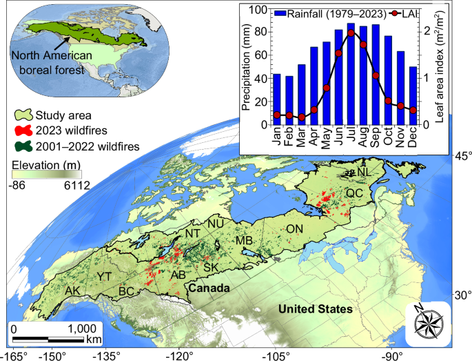
The study area includes North American boreal forests. Historical (1979–2023) monthly precipitation values and MODIS LAI (2000–2023) data are shown in the upper right panel. The precipitation data are based on the National Centers for Environmental Prediction (NCEP) Climate Forecast System (CFS) measurements.
Results
Needleleaf index
We developed a novel spectral index, the NI, for boreal forests based on Landsat infrared bands. The infrared wavelengths were selected for their distinct characteristics: vegetation exhibits high reflectance in the red edge region of the electromagnetic spectrum (0.7–0.8 µm), water shows minimal reflectance in infrared wavelengths, and conifer forests demonstrate lower reflectance in the infrared range (0.85–2.2 µm) compared to other vegetation types. Applying NI to Landsat images makes it possible to distinguish conifer forests from other land covers by applying suitable thresholds.
Needleleaf index threshold
To identify the coniferous forest, an appropriate threshold for the NI was determined. Reference points were selected for each land cover class. The average NI values of the reference points were calculated for each class (Supplementary Fig. 1). By interpreting the Landsat images, the range of NI threshold values for the coniferous forest was considered to be 0.2–0.4 (Supplementary Fig. 1). The maximum and minimum needleleaf forest values were 0.45 and 0.15, respectively, indicating a mixed-pixel problem. According to Supplementary Fig. 1, if the NI value of the pixel was in the threshold range (i.e., 0.2–0.4), the pixel was recognized as a needleleaf forest pixel. Otherwise, the pixel was identified as another land cover type. Pixels with values between 0.15 and 0.2 represented mixed pixels, comprising both coniferous forest and water with different proportions (Fig. 2a). Similarly, mixed pixels containing coniferous and mixed forests had values of approximately 0.4–0.45 (Fig. 2b). Other types of vegetation land cover, including broadleaf forests, croplands, grasslands and shrublands, had values greater than 0.49 and can be well distinguished from coniferous forests.
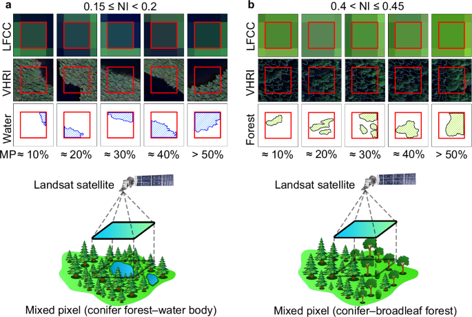
a The mixed pixels (MPs) of water and coniferous forests are observed near the lower range of the NI threshold. The dark and green areas in the very high-resolution satellite imagery (VHRI) panel represent water and coniferous forests, respectively. b The MPs of coniferous and broadleaf forests are observed near the upper range of the NI threshold. The VHRI panel shows that the color and texture of coniferous and broadleaf forests are different. The color of coniferous forests is darker than that of broadleaf forests because of less reflectance in the visible wavelengths. The Landsat false color composite (LFCC) of shortwave infrared (SWIR)-2, near-infrared (NIR), and BLUE is applied to improve the visualization of forest and water phenomena. The percentage of mixed pixels is displayed in detail via VHRI. The schematic diagram of the MP mechanism at the bottom of the figure shows the two mixed pixels of coniferous forest with water and coniferous forest with broadleaf forest.
Needleleaf index mapping results
The results of the needleleaf forest extent maps were derived via the NI (Figs. 3 and 4). The needleleaf forest area maps were prepared after applying the determined NI threshold to Landsat TM, ETM+, and OLI images in the GEE environment. Then, the binary map of the needleleaf forest area was produced at a resolution of 30 m (Fig. 3). Table 1 provides information regarding the CFA extracted from Landsat TM, ETM+, and OLI during the study period (1984–2023). CFA increased steadily from approximately 1.82 million km2 in period 1 to approximately 2.02 million km2 by period 2. The CFA then decreased rapidly, declining to approximately 1.95 and 1.87 million km2 in period 3 and period 4, respectively. The CFA reached 1.92 million km2 by period 5, which was an increase of approximately 54,000 km2 since period 4. There was a significant increase in the CFA, i.e., approximately 102,000 km2, between period 1 and period 5. In the study area, massive wildfires destroyed coniferous forests of approximately 55,205 km2 in 2023. As a result of the wildfires, the coniferous forest area decreased. More precisely, if the wildfires did not occur in 2023, the area of coniferous forests would have increased by 28,474 km2 compared with that in period 3. Supplementary Table 2 summarizes the CFA details shown in the polar bar chart in Fig. 4 for each province.
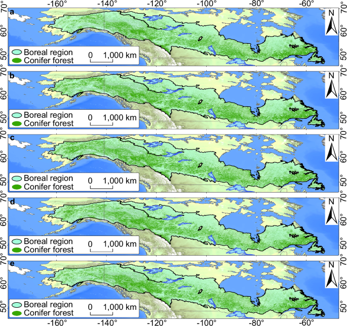
a Coniferous forest cover extracted from Landsat TM satellite images from period 1. b Coniferous forest cover extracted from Landsat TM and ETM+ satellite images from period 2. c Coniferous forest cover extracted from Landsat TM satellite images from period 3. d Coniferous forest cover extracted from Landsat OLI satellite images from period 4. e Coniferous forest cover extracted from Landsat OLI satellite images from period 5.
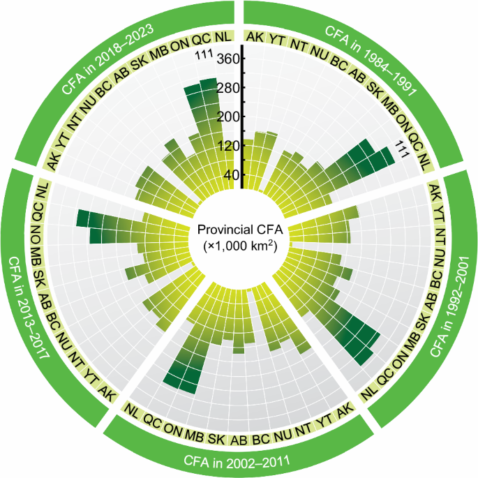
The polar bar chart shows the changes in the coniferous forest area in each province over the five time periods. The numbers on the y-axes (solid black line) represent the CFA in thousand km2. Each part of the diagram depicts a specific study period, and the green gradient bars indicate the CFA in each province.
The CFA in YT, BC, and AB clearly increased between 12% and 29% during period 5. In AK, the CFA increased substantially in period 3 by 63%, after which it decreased gradually until period 5 when it reached 22% above the initial level. In contrast, the CFA in SK, QC, NL, and ON increased steadily from period 1 to period 2, before decreasing below the starting level in period 5 by 1%–9%. The CFA in NU increased moderately over periods 1–3, and then, from period 4, the CFA decreased below the initial level and then increased slowly from period 5. The NT and MB were exceptions. The CFA in the NT increased slightly in periods 1 and 2 and then increased significantly from period 3, followed by a moderate decrease until period 5. The CFA increased by nearly 9% between periods 1 and 5. The CFA in MB fluctuated slowly and eventually increased by approximately 5% compared with that in period 1.
In the study period, the CFA increased the most in the provinces of AB, AK, and BC, with increases of approximately 29%, 22%, and 21%, respectively. Conversely, the maximum decreases in the coniferous forest area were in QC, and NL, with decreases of approximately 9% and 6%, respectively. As a general trend, CFA has increased over time in the western parts of the boreal region, excluding AK. Conversely, in the eastern parts, CFA predominantly shows a decrease. The central parts of the boreal region also exhibit fluctuations in CFA. These results show that destructive activities that destroy coniferous forests are more common in the eastern parts of the boreal region.
Accuracy assessments
The accuracy assessment results for the NI are summarized in Table 2. The error matrices were generated separately for each period. The overall accuracies (OAs) for Landsat TM/ETM+ from period 1, period 2, and period 3 were 91.5%, 91.06%, and 90.2%, respectively, and the kappa coefficients (KCs) were 83.1%, 82.1%, and 80.5%, respectively. The producer accuracy (PA) values for Landsat TM/ETM+ for periods 1–3 were 98.8%, 99.2%, and 98.9%, respectively, and the user accuracy (UA) values for these periods were 85.8%, 85.1%, and 84%, respectively. The OAs for Landsat OLI data from period 4 and period 5 were 90.4% and 89.7%, with producer accuracies of 98.4% and 98.9% and user accuracies of 84.1% and 82.8%, respectively. During these periods, the KCs for Landsat OLI data were 81% and 79.5%, respectively. These results suggest the high confidence level of NI in differentiating needleleaf forests from non-needleleaf forests. The low omission error from the statistical assessment using stratified, randomly distributed samples across the study area indicates that almost all needleleaf forests were mapped precisely, meaning that only 1.2%, 0.8%, and 1.1% were missing from period 1, period 2, and period 3, respectively, and that 1.6% and 1.1% were excluded from period 4 and period 5, respectively. Additionally, there is a low commission error (TM (period 1) = 14.2%, TM/ETM+ (period 2) = 14.9%, TM (period 3) = 16%, OLI (period 4) = 15.9% and OLI (period 5) = 17.2%), which means that approximately 14–17% of the non-needleleaf forests are mapped as needleleaf forests.
The threshold range of 0.15–0.4 was specifically used for water-masked images, as it provided the most accurate results in terms of both overall accuracy and kappa coefficient across all study periods. It is important to note that the 0.2–0.4 threshold is a general range used to extract relatively pure coniferous forest pixels. However, the accuracy of this range is lower compared to the 0.15–0.4 range. This indicates that some coniferous forest pixels present within the 0.15–0.4 range are excluded in the 0.2–0.4 range, resulting in a decrease in accuracy. The 0.2–0.4 threshold range was selected to help isolate pixels that are predominantly composed of coniferous forests, which is important for large-scale analysis. However, the water-masked threshold of 0.15–0.4 was consistently found to yield the best classification performance, minimizing errors associated with mixed pixels and enhancing the overall accuracy of coniferous forest detection (Supplementary Table 3). Reducing the threshold below 0.2 (without water mask) and increasing it beyond 0.4 led to a decrease in classification accuracy, particularly when the proportion of coniferous forests was lower. This trend can likely be attributed to the greater inclusion of mixed pixels and the increased difficulty in distinguishing coniferous forests from other vegetation types at higher thresholds. This distinction is important for understanding how different threshold values impact the classification results, particularly in areas with varying levels of coniferous forest coverage. Furthermore, the use of the water mask played a crucial role in enhancing classification accuracy by removing non-forest areas, particularly water bodies, thereby yielding more accurate and reliable results.
Uncertainty analysis
In order to evaluate the uncertainty associated with conifer forest predictions using the NI spectral index, we performed a Monte Carlo simulation. This approach involved introducing random variations in key input parameters, such as threshold values and NI spectral index values, across multiple iterations of the model. The results showed an average accuracy of 86% with a standard deviation of 0.34, indicating that the model is both accurate and exhibits moderate variability.
The analysis highlights the model’s sensitivity to fluctuations in input data, but the observed uncertainty remains within acceptable bounds, ensuring the robustness of the model. Overall, this uncertainty analysis demonstrates that the model is reliable for conifer forest detection in the study region, with no significant degradation in performance despite the variability in input parameters.
Wildfire assessment
In 2023, a significant amount of the North American boreal forest was burned46,47. The proportion of burned coniferous forest area (BCFA) compared with the total number of fires in 2023 and the CFA in the five time periods are calculated (Fig. 5). The area covered by coniferous forest increased from period 1 until period 2 but then moderately decreased in period 3. The CFA declined continuously until period 4 but then increased to period 5. Although the upward trend in the CFA continued from period 4 to period 5, the CFA in period 5 did not approach its maximum since period 2. The main reason was the occurrence of large-scale fires, especially in 202346,47, which was identified as the largest group of fires since 2001 (Supplementary Fig. 2). More than 55,000 km2 of coniferous forest were destroyed by the 2023 wildfires. These wildfires caused a decrease of 2.79% in the boreal forest area. QC experienced the most significant decline in the boreal forest area, i.e., by 13,737 km2. AB, BC, and the NT experienced successive declines, with decreases of 12,628, 10,193, and 9889 km2, respectively. The lowest BCFAs in the 2023 wildfire area included NU, NL, and AK, with values of 1.8, 19.7, and 239.5 km2, respectively. The highest percentages of BCFAs in the 2023 fire zone were in NU, BC, and MB Provinces, with 79.5%, 67.4%, and 64.6%, respectively. Conversely, NL and AK had the lowest percentage of BCFAs in the 2023 fire season, at 14.7% and 19.3%, respectively. The 2023 wildfires caused significant destruction, particularly in Canadian boreal forests’ eastern and western parts. The coniferous forests in these regions were heavily affected, highlighting the vulnerability of such forested areas to wildfires under certain conditions.
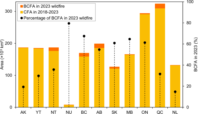
The bars show the conifer forest area (2018–2023) and BCFAs in the 2023 wildfires. The circles show the percentage of BCFAs associated with wildfires in 2023 (the percentage is given on the second y-axis). The BCFA percentage indicates the proportion of burned coniferous forest areas in each province relative to the total burned area in that province during the 2023 wildfires.
Discussion
Monitoring forests in large areas is critical for understanding ecological processes, but it is challenging to perform with remote sensing because of the mixed-pixel problem. The method proposed in this study has been specifically developed to investigate the coniferous forests of North America, which comprise approximately 35% of the world’s largest biome, the taiga. The long-term observations from the Landsat Earth satellite have significantly enhanced regional and global land cover mapping despite the difficulty in distinguishing coniferous forests due to overlapping land covers. We developed a novel spectral index, the NI, for boreal forests based on Landsat satellite observations and computed the CFA across the entire North American boreal biome from 1984 to 2023. Our enhanced NI method is a quicker and more economical way to classify needleleaf forests by differentiation between signals from coniferous forests and other vegetation types. The results revealed that the CFA increased from 1.82 million km2 from period 1 to 2.02 million km2 from period 2 and then decreased to 1.92 million km2 from period 5. High overall accuracies of maps suggest good classification quality; however, it’s crucial to consider additional factors for a comprehensive assessment.
The comparison of the NI, NDVI, and SAVI abilities to detect coniferous forests reveals that coniferous forests can be detected in the NI range of 0.2–0.4 (Fig. 6). This means that the pixels in this range most likely represent coniferous forests. The average NDVI values overlap between needleleaf forest and mixed forest, savanna, broadleaf forest, shrubland, and cropland land covers (dark green arrows in Fig. 6a, b). This result is also somewhat reflected by the SAVI index. Based on Fig. 6, both SAVI and NI indices show nearly similar performance in identifying coniferous forests, mixed forests, and broadleaf forests. However, NI is more efficient than SAVI in detecting coniferous forests. Because, the SAVI values for savanna, shrubland, grassland, and cropland land covers fall within the range of 0.2–0.4 (indicated by the light green arrows in Fig. 6a, b), these land covers may be mistakenly identified as coniferous forests. Identifying coniferous forests via the NDVI and SAVI is difficult because of the overlapping of multiple land covers. The use of the NI has remedied this problem because all land covers have NI values greater than 0.4, except for water bodies, which have NI values less than 0.2. The NI range of 0.2–0.4 highlights only coniferous forests in the boreal biome, which makes it possible to distinguish coniferous forests from other land cover types.
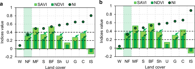
a Landsat TM image. b Landsat OLI image. The horizontal black dotted lines represent the NI index threshold range (0.2–0.4). The light green and dark green arrows show the land covers overlapping with the needleleaf forest and are in the NI index threshold range (0.2–0.4) in the EVI and NDVI, respectively. The horizontal axis shows water (W), needleleaf forest (NF), mixed forest (MF), savanna (S), broadleaf forest (BF), shrubland (Sh), urban (U), grassland (G), cropland (C), and ice and snow (IS) land cover types.
There are similarities between the NI, NDVI, and SAVI. The most significant similarity can be observed in identifying water bodies. The average values of water bodies in the NDVI and SAVI are less than zero. These NI values are positive and close to zero (Fig. 6). Conversely, the major distinction between the NI, NDVI, and SAVI occurs in the snow and ice areas. The NDVI and SAVI values for ice and snow cover are slightly lower than those of water and have the lowest level among land cover types. For the NI, the average ice and snow cover values are greater than those for all land cover types (greater than 0.8). These differences are related to the spectral bands used in the indices. In the infrared range of the electromagnetic spectrum, water has low reflectance48. While snow and ice show high reflectivity in the near-infrared band, their reflectances are low in the shortwave infrared bands.
The NI also has several limitations. The most important restriction is misclassification, which creates an overlap between water bodies and needleleaf forests (Fig. 2a). To overcome this problem, other remote sensing methods can be used49. For example, before applying the NI to satellite images, water areas can be masked49. Under these conditions, the range from 0.15 to 0.4 can be used for detecting coniferous forests. Another limitation of the index is that mountain shade may be mistakenly classified as a coniferous forest in some regions. This error is negligible and does not significantly affect the accuracy of the mapping. Since the mountainous regions don’t extend across the entire boreal region, there are minimal shadows in the Landsat images. Additionally, the near-noon acquisition time of Landsat results in shorter shadows due to the sun’s angle.
The use of the NI for mapping and monitoring boreal forests is very important; because of the large area of this biome and its difficult accessibility, it is not easy to carry out field studies. The NI makes it possible to evaluate the dynamics of boreal forests more quickly and cost-effectively. Furthermore, it allows for an accurate assessment of the extent of forest damage following natural hazards such as fires. The disturbances caused by climate change and wildfires endanger boreal forests12,36. Fires in North American boreal forests have become more common in recent years14. The total burned area, average air temperature, and BCFAs in the boreal zone in North America between 2001 and 2023 are shown in Supplementary Fig. 2. The provinces of SK, QC, NT, AK, and AB have the most burned areas, with 98,811, 93,278, 89,753, 81,425, and 69,621 km2, respectively. In the boreal zone, the provinces of NL and NU experienced the smallest burned areas, with 3909 and 150 km2, respectively. In 2023, the number of fires increased dramatically46,47, burning more than 126,000 km2, which was six times greater than the norm and three times greater than the previous record in 2004. In 2023, the largest fire areas occurred in QC, NT, AB, and BC, with values of 43,491, 27,661, 23,087, and 15,103 km2, respectively. Conversely, the smallest fire areas were in the NU and NL Provinces, with 2.3 and 134 km2, respectively. More precisely, between 2001 and 2023, fires destroyed approximately 218,198 km2 of North American coniferous forests. The highest BCFAs were related to the years 2023, 2004, and 2015, with values of 55,205, 17,465, and 15,510 km2, respectively. The lowest BCFAs were observed in 2001, 2020, and 2022, covering areas of 1239, 505.8, and 93.8 km2, respectively. In the remaining years, BCFAs fluctuated between the mentioned values. The most severe destruction of forests occurred in 2023 when 43.7% of the burned area was composed of coniferous forests. In other words, according to our maps, more than one-quarter of the area of coniferous forest that burned in the last two decades was burned in 2023, and this destruction has been unprecedented since 2001. Severe climatic events, such as El Niño, may result in reduced snow cover, thereby increasing the likelihood of early-season wildfires50, while enhanced snow cover could contribute to the maintenance of soil moisture and mitigate the risk of wildfires.
Since 2001, the average air temperature in the North American boreal zone has been rising, despite substantial fluctuations (Supplementary Fig. 2). The average temperature of the boreal region from 2001 to 2022 was −2.6 °C. The average air temperature in 2023 reached −0.78 °C, which was 0.4 °C warmer than the previous high temperature recorded in 2010. Furthermore, the temperature was 1.8 °C above the average air temperature, which was the highest in the last 23 years. This occurrence could be a result of global warming and its implications.
The method proposed in this study can also be implemented in the coniferous forests of Northern Eurasia. However, additional validation across diverse ecosystems is needed to assess its robustness. Further research will enhance the applicability of the NI to other regions within the taiga biome and improve our understanding of its spatial and temporal variations. To improve the accuracy of boreal forest cover classification, the use of hyperspectral satellite imagery is recommended. Additionally, the application of the NI index could be extended to high-resolution multispectral satellites, such as Sentinel-2, which acquire infrared band images.
Methods
Landsat Collection-2 surface reflectance product
The Landsat satellite series was launched by the National Aeronautics and Space Administration (NASA) and the U.S. Geological Survey (USGS). Landsat acquires global medium spatial resolution images of the Earth’s surface and provides multispectral observations23,26,51. This study used Landsat 5, 7, and 8–9 Collection 2 Level-2 Science Products at a 30-meter spatial resolution (Supplementary Table 1).
Landsat Operational Land Imager (OLI) Collection 2 Level-2, Landsat 5 Thematic Mapper Collection 2, and Landsat 7 Enhanced Thematic Mapper Plus Collection 2 are derived from the data produced by the Landsat OLI/Thermal Infrared Sensor (TIRS), TM, and ETM+ sensors, respectively, and contain atmospherically corrected surface reflectance (SR) and land surface temperature data. Landsat 8 SR products are created with the Land Surface Reflectance Code (LaSRC)52. Landsat 5 and 7 SR products are created with the Landsat Ecosystem Disturbance Adaptive Processing System (LEDAPS) algorithm53.
Several factors were considered when the images were selected. First, the cloud and snow cover had to be less than 10% in the Landsat scenes. To ensure optimal conditions for change detection, imagery should ideally be collected under clear skies with minimal cloud cover54. In less ideal atmospheric conditions, some images may need to be excluded from further analysis54. According to the atmospheric conditions of the study area, cloudless images were obtained in the summer. Second, the vegetation had to have grown enough to be detected in images. We created cloud-free composites for Landsat images from 1984–1991, 1992–2001, 2002–2011, 2013–2017, and 2018–2023 via all available summer images (June–September) from the TM, ETM+, and OLI sensors (Supplementary Table 1).
The LAI was estimated from the 8-day Moderate Resolution Imaging Spectroradiometer (MODIS) LAI product (MOD15A2H V6.1), with a 500-m spatial resolution. The MOD15A2H MODIS combined the LAI and fraction of photosynthetically active radiation (FPAR) products. The extent of burned areas was calculated between 2000 and 2023 from the MODIS MCD64A1 Version 6.1 Burned Area data product on the GEE platform. The MCD64A1 dataset is a monthly dataset at a 500-meter resolution and combines MODIS surface reflectance data with 1 km MODIS active fire observations. Landsat images were used to calculate the burned coniferous forest area each year. The annual burned area was extracted from MCD64A1. The coniferous forest in this area was then estimated by applying the NI index to the prefire Landsat satellite images.
ERA5-Land was used to obtain the average annual precipitation and air temperature data55. ERA5-Land is a reanalysis dataset that combines model data and global observations to provide realistic climatic descriptions of land variables over several decades.
Reference point dataset for determining the threshold
All processing was performed on the GEE platform, and on-the-fly point drawing capabilities were used over the background of the submeter to 5-m VHRI to add the reference samples as needed. In the next step, reference data were collected and labeled with ten class names using historical images from Google Earth Pro VHRI, the MODIS land cover product, aerial photography, and ancillary information from expert judgments (Supplementary Fig. 3). Each reference sample was selected via a random sampling design (Supplementary Fig. 4). In total, during the study period, 13,719 reference sample points were generated separately for the TM and OLI sensors (Supplementary Table 4).
Needleleaf index development
This study developed a new spectral index using Landsat infrared bands. The NI is a new spectral index developed to identify needleleaf forests in Landsat satellite images. The NI was calculated as follows:
where ρNIR, ρSWIR1 and ρSWIR2 are the reflectances of the near-infrared, shortwave infrared-1 and shortwave infrared-2 bands, respectively. For Landsat 8–9, this equation is as follows:
In Eq. 2, NIOLI is the needleleaf index for the Landsat OLI sensor, B5 is the near-infrared band (wavelength = 0.85–0.88 μm), B6 is the shortwave infrared-1 band (wavelength = 1.57–1.65 µm) and B7 is the shortwave infrared-2 band (wavelength = 2.11–2.29 µm). For Landsat 5 TM and Landsat 7 ETM + , Eq. (1) is written as follows:
In Eq. 3, NITM&ETM+ is the needleleaf index for Landsat TM and Landsat ETM+, B4 is the near-infrared band (wavelength = 0.77–0.90 μm), B5 is the shortwave infrared-1 band (wavelength = 1.55–1.75 µm) and B7 is the shortwave infrared-2 band (wavelength = 2.09–2.35 µm).
For developing the NI, the wavelengths were selected according to the following criteria:
-
Vegetation has high absorbance (low reflectance) in the visible range (0.4–0.7 µm) and very high reflectance in the NIR region54.
-
Pure water has low reflectance over the visible, NIR, and SWIR regions48. For pure water, there is almost no reflectance at infrared wavelengths.
-
Compared with other vegetation covers, needleleaf forests have low reflectance in the infrared range (0.85–2.2 µm)5,56 (Supplementary Fig. 4).
There is significant redundant spectral information in OLI bands 1, 2, 3, and 4, as indicated by their strong correlation (r > 0.8) (Supplementary Table 5). Although not to the same degree, the reflective and middle-infrared bands (5, 6, and 7) display significant redundancy, with correlations ranging from 0.11 to 0.86. The lowest correlations occur when a visible band is compared with an infrared band, particularly for bands 1 and 5 (r = 0.06). Band 5 is the least redundant infrared band compared with all four visible bands (1, 2, 3, and 4). The TM bands also show a similar trend (Supplementary Table 6). Therefore, to discriminate between needleleaf forests and other vegetation cover types, the ideal portions of the spectrum for remote sensing are the near-infrared (0.85–0.88 µm) and shortwave infrared (1.57–1.65 µm and 2.11–2.29 µm) regions. Needleleaf forests reflect less than 20% of the incident near-infrared energy (Supplementary Fig. 4).
To obtain the average spectral characteristics of vegetation classes, hundreds of pixels in each class were selected, and the average spectral reflectance was calculated (Supplementary Table 4). The spectral values of different land covers in the Landsat imagery in the visible bands (blue, green, and red) are almost the same, but they are distinguishable in the NIR and SWIR bands (Supplementary Fig. 4). Additionally, the spectral values of the broadleaf trees are greater than those of the coniferous trees. Therefore, the infrared bands (NIR and SWIR) were considered the best bands for discerning needleleaf forests. A schematic of the data preprocessing, NI index development, and estimation of the coniferous forest area via the NI is presented in Supplementary Fig. 5.
Decision Tree classification
We employed a Decision Tree (DT) model for the classification process. The DT is a widely used machine learning algorithm due to its simplicity, interpretability, and ability to handle both categorical and continuous data. The DT model was applied to classify the Landsat images into coniferous forest and non-coniferous forest categories. The model was developed within the GEE environment through the implementation of JavaScript code. Initially, the DT model was implemented by masking water bodies using the Normalized Difference Water Index (NDWI) index49. Then, a rule based on a threshold range of 0.15–0.4 was applied to extract coniferous forest areas. The output was a binary image of coniferous forest and non-coniferous forest.
Accuracy assessments by using validation samples
It is possible to estimate the accuracy of remote sensing thematic maps by comparing the classified map and reference information. This comparison was performed in the error matrix. The initial results of coniferous forest mapping for the Landsat images were evaluated using approximately 30,000 validation samples. The validation dataset for this study was created by randomly selecting points across the North American boreal biome (Supplementary Fig. 6). The validation points are uniformly distributed across the region, encompassing various conifer species. To classify each point as coniferous forest or non-coniferous forest, we utilized a combination of datasets, including aerial photographs, the MODIS land cover product (MCD12Q1)57, the European Space Agency Global Land Cover Map58, and high-resolution multitemporal imagery from Google Earth Pro, provided by Airbus and Maxar. Approximately 15,000 points were selected for coniferous forests, with an approximately equal number for non-coniferous forests. These points were carefully validated using the datasets mentioned earlier. During the five study periods, the reference points were reviewed and updated, when necessary, with some points being adjusted or removed due to minimal land cover changes.
For the western sections of the study area (Alaska), high-resolution aerial photographs were used for the periods 1–3 (1984–2011). The scale of the aerial photographs used in this study ranged between 1:3000 and 1:30,000. These photographs include two datasets: Aerial Photo Single Frames Records59 and High Resolution Orthoimagery (HRO)60.
The Aerial Photography Single Frame Records collection contains millions of aerial photographs taken by federal agencies59. These data were used from 1984 to 2008 and are accessible for download in both medium and high resolutions through the USGS Earth Resources Observation and Science (EROS) archive. The collection primarily covers the United States, as well as parts of Central America and Puerto Rico. Aerial photographs are available in black-and-white, natural color, and color infrared formats for the United States. These aerial photographs were used to generate validation points for the periods 1–3.
High-resolution orthorectified images combine the detailed visual qualities of aerial photographs with the geometric accuracy of maps60. Managed and distributed by the USGS EROS Center, this orthoimagery is available in several formats, including black-and-white, natural color, color infrared, and color near-infrared. These digital orthorectified aerial photographs, with a pixel resolution of 1 meter or finer, cover extensive areas across the United States from 2000 to 2016. These aerial photographs were usable in the study area for period 3.
The land cover layer was derived from the Terra and Aqua combined MODIS Land Cover Type (MCD12Q1) Version 6.1 data product at 500 m resolution57. This dataset was utilized to generate reference points for the periods 3–5 (2002–2023). Due to the large pixel size of this product, the coniferous forest pixels were examined by visual interpretation of the high-resolution images in Google Earth Pro. Only the pixels that accurately represented coniferous forests were selected for analysis.
Additionally, we used the Global Land Cover Map dataset, a global land cover map based on ENVISAT’s Medium Resolution Imaging Spectrometer (MERIS) Level 1B data58, with a spatial resolution of approximately 300 meters, for period 3. This land cover map is generated through an automated, regionally-tuned classification of a time series of global MERIS mosaics from 2009. The map includes 22 land cover classes, defined according to the United Nations (UN) Land Cover Classification System (LCCS). Here, we also examined the pixels to distinguish pure land cover types in order to extract the validation points.
For periods 2–5, we used Google Earth Pro images to extract accurate validation points. The validation points from period 2 were also applied to period 1, as they were specifically selected to represent mature, dense coniferous forests. This approach ensured that the same points in period 1 corresponded to coniferous forests as well. The high-resolution images, including data from Airbus and Maxar, provided detailed and precise information, enabling the identification of reliable validation points for land cover assessment. With a resolution of approximately 30 centimeters, these high-quality images were particularly useful for distinguishing and confirming land cover types at finer scales. An additional advantage of this dataset is that it provides images from multiple years, allowing for temporal comparisons and more robust validation across different time periods.
The overall accuracy of the classification was obtained by dividing the diagonal elements of the error matrix (correctly classified pixels) by the total number of pixels in the error matrix61,62. The PA and UA were also calculated to evaluate the classification performance. The PA is the total number of correctly classified pixels in each class divided by the total number of reference data in that class62. The UA is the total number of correctly classified pixels in a class divided by the total number of pixels of the same class in the classified map62. The PA and UA are adequate indicators of how well a classification category has been classified. We also calculated a kappa statistic, which is a discrete multivariate technique used for accuracy assessment63.
Monte Carlo simulation for uncertainty analysis
To assess the uncertainty in the coniferous forest detection results, we employed a Monte Carlo simulation approach64. This method involves generating random variations in key input parameters and running the model multiple times to evaluate the impact of these variations on the prediction accuracy. The key input parameters for the Monte Carlo simulation included:
-
Threshold values used to classify pixels as coniferous forest or non-forest.
-
NI Spectral index values derived from the Landsat bands.
Each simulation run involved randomly varying these parameters within a defined range (e.g., ±5% for threshold values, ±10% for spectral index values) to simulate real-world variability.
The simulation was run 2000 times, and for each iteration, the model’s prediction accuracy was calculated. The results of the simulations provided a distribution of outcomes for each of the key metrics. After running the simulations, we calculated the mean and standard deviation of the prediction accuracy across all iterations. This analysis allowed us to quantify the uncertainty associated with the model’s predictions.
Responses