Gene regulatory network inference during cell fate decisions by perturbation strategies

Cell fate decision, a complex dynamical process involved in the whole life, is intricately regulated by various molecules¹. The transitions between distinct cell fates, such as differentiation, reprogramming, or transdifferentiation, occur during developmental processes^2,3. The dynamical variations of various cell fates can be quantitatively captured through gene regulatory networks^4,5,6,7. However, despite these advancements, accurately identifying the regulations and their intensities involved in these networks using solely in vivo experimental data is still difficult^8,9,10. Consequently, inferring gene regulatory networks based on data sources remains a fundamental yet unresolved problem in systems biology.

In the realm of biological systems involving cell fate decisions, several methods have been developed to characterize cell fates using single-cell RNA sequencing (scRNA-seq) data, e.g., TSCAN¹¹, Monocle 2¹², SPRING¹³, and Slingshot¹⁴. In addition, the distance covariance entropy (DICE) approach has the ability to predict regulatory factors underlying various phenotypes¹⁵. However, these methods often encounter limitations in inferring topological structures of gene regulatory networks associated with identified cell fates, i.e., even with the ability to determine cell states, network topologies of the system remain unknown.

On the other hand, there are algorithms for gene regulatory network inference using scRNA-seq data based on mutual information, random forest, correlation, regression, ordinary differential equations (ODEs), or Boolean models. Examples of such algorithms include PIDC¹⁶, GENIE3¹⁷, PPCOR¹⁸, SCODE¹⁹, and SCNS²⁰. However, each of these network inference algorithms possesses its specific limitations. For example, PIDC and PPCOR fail to capture the directionality of regulations, while GENIE3 is limited to identifying the existence of regulations without quantifying their strength or weight. For SCODE, regulatory networks can only be inferred when specific linear ODEs with known parameters are employed, and these parameters can be further refined through linear regression and error iteration. In contrast, for the SCNS algorithm, the network model based on Boolean local rules can only be reconstructed if the three parameters corresponding to each gene are predetermined. Unfortunately, none of these methods adequately account for the dynamical network differences during cell fate decisions.

Modular response analysis (MRA) is an effective approach for inferring network connections through the analysis of experimental data obtained from various perturbations. Within this framework, the local response matrix provides a quantitative representation of both the direction and intensity of the interconnected edges within the network²¹. This indicates that the local response matrix has the potential to provide significant insights into biological network topologies. However, MRA failed to account for network topological variations across different cell states and the network inferred using local response matrix dose not satisfy the sparsity requirement of regulatory networks. In addition, there is still a gap in understanding the effects of different perturbation degrees on local response matrices^22,23.

Here, we introduce a computational method aimed at inferring network topologies and identifying differences among networks during cell fate decisions. This method is achieved through statistical and differential analyses of expression data subjected to systematic perturbations. Our method is broadly applicable and theoretically suitable for a variety of expression data types, including single-cell gene expression data, experimentally obtained measurements, or stable cellular data derived from software simulations. In addition, there are no restrictions on the scale of the inferred networks. Initially, local response matrix at each cell state is numerically calculated from perturbation data. The elements within the matrix correspond to regulations between molecules, meaning that local response matrix reveals network topologies associated with cell fate decisions. Furthermore, based on statistical analysis, the confidence intervals (CIs) of local response matrix are employed to identify the sparsity of regulatory networks^24,25, as well as the influence of regulation degrees. Subsequently, we construct the redefined local response matrix to reflect the network topologies during all cell states, and the accuracy of the inferred network topologies can be verified by two types of errors. Furthermore, differential analysis is performed to determine the relative local response matrix, thereby quantifying critical regulations within each cell fate and identifying primary cell states associated with specific regulations.

To demonstrate the feasibility of our approach, we choose the epithelial to mesenchymal transition (EMT) network as an illustrative example²⁶. This example demonstrates how perturbation and statistical analyses are applied to infer regulatory networks, how differential analysis is performed to identify critical regulations in three distinct cell states: epithelial (E), mesenchymal (M), and hybrid (H) state with both E and M features, and how specific cell states related to each regulation are determined. For the analysis of EMT network, we utilize mathematical model (ODEs) to simulate systematic perturbations and obtain the expression data of all molecules. However, it is worth noting that our approach is theoretically applicable to measured experimental data as well. Additionally, the calculation of local response matrices, which is based on data, is model-independent. We demonstrate the feasibility of our method by comparing it with priori knowledge^{27,28,29,30,31}, indicating its capability in inferring network topologies and identifying network differences.

Fundamentals of the network inference

For a gene regulatory network comprised of n molecules, i.e., nodes, and multiple molecular regulations, i.e., links or edges, the dynamics of the network can be generally described by a set of ODEs as follows

where ({{boldsymbol{x}}}={({x}_{1},cdots ,{x}_{n})}^{T}) is a time-dependent vector representing concentrations of the molecules, such as genes or proteins, ({{boldsymbol{f}}}={({f}_{1},cdots ,{f}_{n})}^{T}) is a continuously differentiable function vector related to the production and consumption of the molecules as well as the regulations between them, and p = (p₁,…, p_u, p_u+1,…, p_m), m > u ≥ n, is a parameter vector including rate constants, Michaelis constants, etc.

To infer network topologies and investigate network differences across different cell fates based on perturbation analysis, we divide p into two parts, the sensitive parameter set (p₁,… p_u) and the constant parameter set (p_u+1,…,p_m). The sensitive parameter set can be perturbed and is associated with nodes, each of which contains at least one sensitive parameter, such as the basic generation rate, degradation rate, signals pertinent to the specific node, or activators and inhibitors. The perturbation applied to the sensitive parameter associated with node i meets the criterion that the expression of node i is initially and directly influenced by this perturbation, with subsequent indirect effects on the expressions of other nodes due to the regulations among them. Here, we restrict our analysis to each node contains only a single sensitive parameter, i.e., u = n, ∂f_i/∂p_i ≠ 0, and ∂f_i/∂p_k = 0, 1 ≤ i ≠ k ≤ n.

We assume the system (1) reaches a locally stable steady state (bar{{{boldsymbol{x}}}}=({bar{x}}_{1},cdots ,,{bar{x}}_{n})) at the basal unperturbed sensitive parameter set p_b = (p_b,1,…, p_b,n) and the constant parameter set p_c = (p_c,n+1,…, p_c,m), i.e.,

In other words, (bar{{{boldsymbol{x}}}}) represents an unperturbed stable steady state at the unperturbed sensitive parameter set p_b and the constant parameter set p_c. Denote the perturbed stable steady state by ({bar{{{boldsymbol{x}}}}}_{k}=({bar{x}}_{k,1},cdots ,,{bar{x}}_{k,n})) after sensitive parameter p_k is slightly perturbed from p_b,k to p_s,k. Define p_s = (p_s,1,…, p_s,n) as the perturbed sensitive parameter set. Here, (bar{{{boldsymbol{x}}}}) and ({bar{{{boldsymbol{x}}}}}_{k}) must be the same type of cells, and ({bar{x}}_{i}ne 0), ({bar{x}}_{k,i}ne 0), i, k = 1,…, n.

The direct regulation from node j to node i can be quantified by the relative change of (Delta {x}_{i}/{bar{x}}_{i}) with respect to (Delta {x}_{j}/{bar{x}}_{j}) under the mild perturbation of sensitive parameters. It is defined as local response coefficient r_ij, i.e.,

where Δx_i represents the change of ({bar{x}}_{i}) under the perturbation to one sensitive parameter, and we define r_ii = − 1. The sign of r_ij reflects the type of regulation from node j to node i, the absolute value of r_ij indicates the strength of the regulation, where r_ij > 0 (or r_ij < 0) represents activated (or inhibitory) regulation, and r_ij = 0 indicates no direct regulation from node j to node i, i ≠ j. Meanwhile, the relative change of node i to the change of an infinitesimal perturbation for a sensitive parameter p_k defines the global response coefficient R_ik, i.e.,

We use r = (r_ij) and R = (R_ik) to represent the local response matrix and the global response matrix²¹, respectively. Therefore, the local response matrix r can be used to characterize the network topology of the system.

The relationship between local response matrix and global response matrix

Usually, a slight perturbation to p_k initially affects node k, and subsequently propagates to node i via both direct regulation from k to i and indirect path from k to i, which includes intermediate nodes. Therefore, it is impractical to determine the precise proportion of direct and indirect regulations that contribute to the ultimate change in node i under the perturbation p_k. In other words, the local response matrix r can not be measured directly based on the experimental data before and after perturbations. However, the global response matrix R can be calculated directly.

In experimental measurements, based on the work of literature²¹, the global response coefficient R_ik can be quantitatively expressed as (Delta ln {x}_{i}(k)/Delta ln {p}_{k}), where (Delta ln {x}_{i}(k)=ln {bar{x}}_{k,i}-ln {bar{x}}_{i}) and (Delta ln {p}_{k}=ln {p}_{s,k}-ln {p}_{b,k}). Using central difference approximations and ignoring the higher order nonlinear terms for the logarithmic function, we have

Based on the multivariate implicit function theorem and the multivariate chain rule, the local response matrix r is related to the global response matrix R (see Method or equation [5] in ref. ²¹), i.e.,

Consequently, utilizing only the data obtained before and after perturbations to sensitive parameters, without the need for specific ODEs and regardless of the network size, the local response matrix r can be directly inferred from equations (2) and (3). We refer to the analysis involving perturbations to sensitive parameters as systematic perturbation analysis. Therefore, network topologies and regulation strength at each cell state can be inferred. It is important to note that the calculation of r is only valid when the data obtained after perturbations are in close proximity to the unperturbed stable steady states, i.e., there is no qualitative differences in these data (no transition from one cell state to another).

Additionally, when the ODEs and corresponding parameter values of system (1) are known, we can get

where the Jacobian matrix J at the stable steady state (bar{{{boldsymbol{x}}}}) takes the form

and the nonsingular diagonal matrix ({{boldsymbol{X}}}={{rm{diag}}}(bar{{{boldsymbol{x}}}})) (see Method). Therefore, the local response matrix r at (bar{{{boldsymbol{x}}}}) can also be calculated when the Jacobian matrix J (or specific ODEs) of system (1) at (bar{{{boldsymbol{x}}}}) is known. For simplicity and to distinguish r computed by Eqs. (2) and (3), we call the local response matrix obtained by Eq. (4) as the wild-type (WT) local response matrix, denoted as r⁰.

However, obtaining ODEs and their corresponding parameter values which accurately represent a gene regulatory network is often challenging in practice, making the calculation of r⁰ impractical. Fortunately, experimental measurements of the data before and after systematic perturbations are feasible, allowing for the calculation of r using Eqs. (2) and (3).

The inference of network topologies and identification of network differences

There are numerical inaccuracies in deriving r through the utilization of the cell data before and after sensitive parameter perturbations, mainly due to fluctuations in actual measurements caused by internal and external environmental factors and the difference in perturbation intensity of sensitive parameters. Additionally, the omission of higher-order nonlinear terms (central difference approximation) further contributes to the inaccuracies. Furthermore, the majority of elements in r calculated using Eqs. (2) and (3) are nonzero (see ref. ²¹), which is contradict with the sparsity of regulatory networks. Consequently, it is imperative to diminish the significance of most predicted regulations to minimize the disparity between the inferred and the true networks, thus reducing the inaccuracy.

Based on perturbation and statistical analyses, we construct the redefined local response matrix (hat{{{boldsymbol{r}}}}=({hat{r}}_{ij})) to reflect the network topologies more accurately (see Methods). For a gene regulatory network with s different cell fates, there are s redefined local response matrices, i.e., one (hat{{{boldsymbol{r}}}}(v)) for the v-th state, v = 1,…, s. And there exist quantitative variations in the network topologies for these s cell fates. Further, based on differential analysis, we define the relative local response matrix (widetilde{{{boldsymbol{r}}}}(v)=({widetilde{r}}_{ij}(v))) to quantify the differences of the regulations across all cell fates (see Methods).

In summary, to infer network topologies and identify network differences across all cell fates, the specific steps are as follows.

1. 1.

   Determine nodes and their respective sensitive parameters. Additionally, identify the number of cell fates present within the network. Assume the network has n nodes and s different cell fates, with each node having only one sensitive parameter. For each cell fate, measure unperturbed steady state data (bar{{{boldsymbol{x}}}}(v)) under unperturbed sensitive parameter set p_b(v), v = 1, …, s.

2. 2.

   Randomly select values for one perturbed sensitive parameter set p_s(v) from distributions such as the uniform or normal distribution under systematic perturbation analysis. Calculate the global response matrix R(v) by Eq. (2) and using the measured stable steady state data before and after perturbations. Then, infer the local response matrix r(v) by Eq. (3).

3. 3.

   Repeat step 2 multiple times to obtain the distribution of r_ij(v) and then verify whether the 95% confidence interval (CI) of the distribution contains zero for all 1 ≤ i ≠ j ≤ n in statistical analysis. Further, infer the redefined local response matrix (hat{{{boldsymbol{r}}}}(v)) which reveals network topologies across all s cell fates.

4. 4.

   Calculate the relative local response matrix (widetilde{{{boldsymbol{r}}}}(v)) based on (hat{{{boldsymbol{r}}}}(v)) in differential analysis, which serves as a quantitative tool to identify and compare network differences across all cell fates.

Application to the EMT network

To demonstrate feasibility of the approach, we apply it to the EMT network²⁶. The approach presented here can be applied to diverse biological systems, enabling the inference of network topologies and the identification of crucial network differences across various cell fates.

EMT plays crucial roles in both physiological and pathological processes, such as tissue repair, normal embryonic development, wound healing, and cancer metastasis^32,33,34. During EMT, epithelial cells undergo a morphological transformation characterized by the loss of cell-cell polarity and adhesion, ultimately transforming into mesenchymal cells with enhanced motility and invasive capabilities. A hybrid phenotype exists during this transition process^35,36,37. Consequently, the EMT process involves three stable steady states: the epithelial (E) state, the hybrid (H) state, and the mesenchymal (M) state^38,39.

The core EMT network is composed of nine molecules, including one endogenous transforming growth factor-β (TGF-β), two transcription factors, SNAIL1 and ZEB, two mRNAs, snail1 and zeb, two microRNAs, miR-34 and miR-200, and two markers, E-cadherin and N-cadherin, as shown in Fig. 1. TGF-β promotes the transcription of snail1 mRNA, which is translated to SNAIL1⁴⁰. SNAIL1 promotes the expression of zeb mRNA, which is translated to ZEB⁴¹. Both SNAIL1 and ZEB repress the transcription of miR-34 and miR-200. In turn, miR-34 and miR-200 inhibit the expression of SNAIL1 and ZEB, respectively^42,43. In addition, miR-200 also suppresses the expression of TGF-β⁴⁴. SNAIL1 and ZEB inhibit the expression of E-cadherin and promote the expression of N-cadherin.

Green arrows and red bars denote activation and inhibition, respectively.

Full size image

Detailed ODEs of the dynamical model are given in Supplementary Note 1. Since E-cadherin and N-cadherin do not affect the expression of other molecules, namely, there is no regulation from them to other molecules, we exclude them in the following analysis. That is, only 7 nodes and 11 regulations are left. The details on all regulations are given in Table 1. By using the parameters in Supplementary Note 2 (Supplementary Table 1) to solve the ODEs under different initial conditions, the expression data of the three stable phenotypes, E, H, and M, can be calculated concretely. The diagonal matrix X(v) constituted by expressions of the seven molecules at each state and the corresponding Jacobian matrix J(v) can be obtained, where v = 1, 2, 3 represents E, H, and M states, respectively.

Inferring the EMT network

To infer network topology across all cell fates based on perturbation and statistical analyses, i.e., to derive the redefined local response matrix (hat{{{boldsymbol{r}}}}(v)) using the stable steady state data before and after perturbations, instead of relying on specific ODEs and parameter values of the system, we initially determine the set of sensitive parameters (kd₁,…, kd₇), which comprised by the degradation rates of all nodes. This set satisfies that a perturbation to kd_i directly affects only the expression of node i, and subsequently, indirectly alters the expression of other nodes, i = 1,…, 7 represent TGF-β, snail1, SNAIL1, miR-34, zeb, ZEB, and miR-200, respectively. Once the perturbed sensitive parameter set is determined, the local response matrix can be calculated by using only the measured stable data before and after perturbations to sensitive parameters.

Since the local response matrix calculated from one perturbed sensitive parameter set may have randomness and contingency, we adopt a resampling approach to mitigate these effects. By repeatedly perturbing the sensitive parameter set 2000 times and calculating the corresponding local response coefficients for each set, i.e., N = 2000, we obtain these resampling local response matrices. For each perturbed sensitive parameter set, we assume it follows either a uniform or normal distribution. Recognizing that the perturbation levels applied to sensitive parameter set can lead to differences in measured data, which may further cause differences in calculated local response matrices, we select two distinct perturbation levels for each distribution: 20% or 50% for the uniform distribution (Type I or II), and 10% or 20% for the normal distribution (Type III or IV), the details of each perturbation are outlined in Table 2.

By applying statistical analysis to these resampling local response matrices, we can derive the distribution of each local response coefficient and its corresponding 95% CI. Among them, only certain elements of r(v) satisfy the criterion: 0 does not fall within the 95% CI. The diagonal elements of r(v), − 1, are excluded in the following analysis. For these four perturbations, the probability distribution of calculated local response coefficients satisfying the criterion are shown in Fig. 2. Obviously, the total count and the intensities of identified regulations differ in E, H, and M states. For each state, the disparity of the total count is mainly caused by elements approaching zero. The closer the calculated local response coefficient r_ij approaches zero, the more significant the differences become, e.g., r₇₆ in E state and r₇₃ in H state. For the distributions of r_ij satisfying 0 ∉ the 9 5% CI across all the four perturbation types, there exist minor disparities near the left and right endpoints of these distributions at each state, and the distribution associated with each perturbation type exhibit distinct patterns, satisfying the principle that as the perturbation degree increases, the distribution tends to become more gradual.

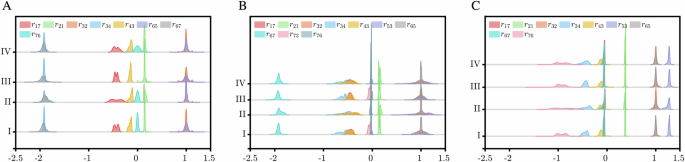
The horizontal axis depicts the values of r_ij, while the vertical axis represents corresponding distribution frequency.

Full size image

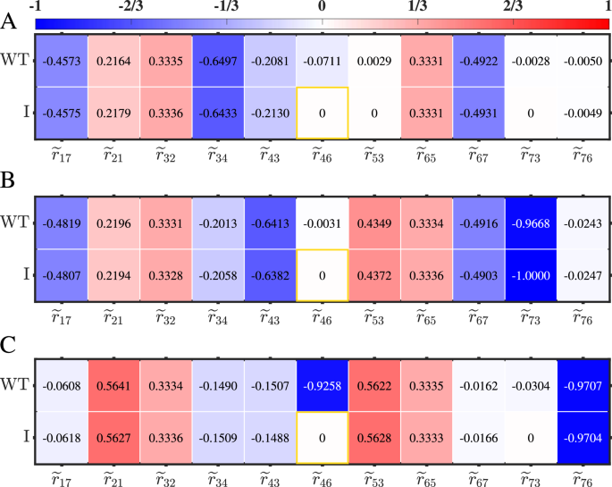
At each state and for each perturbation type, the number of non-zero elements in the redefined local response matrix (hat{{{boldsymbol{r}}}}(v)) equals the total number of probability distributions identified in Fig. 2, i.e., most elements are zero and only some elements are non-zero. To assess the accuracy of (hat{{{boldsymbol{r}}}}(v)), which is calculated using Eqs. (2), (3), (6), in reflecting the true network topologies, we calculate the wild-type (WT) local response matrix r⁰(v) based on Eq. (4) for comparison. Only some elements of r⁰(v), corresponding to true regulations listed in Table 1, are non-zero, and the value and sign of ({r}_{ij}^{0}) reflect the regulatory information on L_ij. To verify the effects of perturbation degrees and distributions on (hat{{{boldsymbol{r}}}}(v)), as well as to characterize the difference between the redefined and WT local response matrices, the contrast between the non-zero elements in r⁰(v) and corresponding elements in (hat{{{boldsymbol{r}}}}(v)) under four perturbation types is shown in Fig. 3.

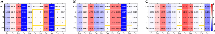
Each element’s value is depicted by a distinctively colored box, with the intensity of the color indicating the strength of the regulation. Specifically, a positive value denotes activation, whereas a negative value denotes inhibition. This contrast reflects the difference between true and inferred networks. The top row represents the non-zero elements of the WT local response matrices. The elements satisfying ({hat{r}}_{ij}(v)=0) are marked by orange boxes.

Full size image

When ({r}_{ij}^{0}(v)) significantly deviates from zero, corresponding ({hat{r}}_{ij}(v),ne, 0) and fluctuates around ({r}_{ij}^{0}(v)) under four perturbation types, i.e., there is a slight difference between ({hat{r}}_{ij}(v)) and ({r}_{ij}^{0}(v)) quantitatively. However, for ({r}_{ij}^{0}(v)) close to zero, corresponding ({hat{r}}_{ij}(v)) may either be zero or extremely close to ({r}_{ij}^{0}(v)) and be non-zero under four perturbation types, i.e., a few elements exhibit qualitative differences. Specifically, the actual regulation from ZEB to miR-34 exists in all cell phenotypes, i.e., ({r}_{46}^{0},ne, 0), while we obtained ({hat{r}}_{46}=0) at each perturbation analysis. The main reason for this difference we considered is that the value of ({r}_{46}^{0}) at each state is very close to zero, resulting in the 95% CI of r₄₆ under resamplings including zero, the same for the regulation from SNAIL1 to zeb in E state (i.e., r₅₃(v), v = 1), and almost the same for the regulation from SNAIL1 to miR-200 (i.e., r₇₃), with the only difference is that ({hat{r}}_{73},ne, 0) in H state and for the perturbation types I and type III (small degree of perturbation).

When the true element ({r}_{ij}^{0}(v)) is far from zero, the perturbation degrees and distributions barely alter ({hat{r}}_{ij}(v)). Conversely, if ({r}_{ij}^{0}(v)) is exceedingly small, the perturbation degrees may significantly affect the identification of regulations. Specifically, a smaller perturbation degree results in a more precise identification of regulations, while the distribution type of perturbation has little effect on the identification. Consequently, the network topologies inferred from perturbation data closely resemble the true network topologies obtained based on the dynamical model across all the three cell states, although the regulations inferred from four perturbation types exhibit subtle differences in each state.

To verify whether the redefined local response matrix (hat{{{boldsymbol{r}}}}) can be used to reflect the WT local response matrix r⁰, i.e., how precisely the inferred network topologies based on stable steady-state data before and after perturbation capture the true network topologies, we compute two types of errors. One is the inference error between (hat{{{boldsymbol{r}}}}) and r⁰, (hat{e}=sqrt{{sum }_{i,j}{({hat{r}}_{ij}-{r}_{ij}^{0})}^{2}}). The other is the sample error between r^l and r⁰, ({e}_{l}=sqrt{{sum }_{i,j}{({r}_{l,ij}-{r}_{ij}^{0})}^{2}}), l = 1,…, N. The two types of errors for each state under the four distinct perturbation types are presented in Fig. 4. In each state, the colored dots (green, orange, blue, and yellow dots) represent the values of e_l for resamplings under four perturbation types, which form violin-shaped distributions to illustrate the sample errors across all perturbation types. The corresponding red dot marks the mean of each distribution, while the error bar indicates its standard deviation. Additionally, the red + sign positioned at each distribution represents the value of (hat{e}(v)).

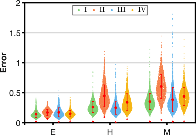
The inference errors are represented as the red + signs. The sample errors under perturbation type I, II, III, and IV are represented as green, orange, blue, and yellow dots, respectively.

Full size image

Obviously, there is some examples with significant sample errors within each distribution, although majority clusters around the mean of distribution, suggesting that the inferred regulations under a single perturbation set may deviate substantially from the true network. Moreover, as perturbation degree increases, the sample errors tend to grow larger. Specifically, the majority of sample errors under perturbation type II, depicted by orange dots, are generally higher than those under other perturbation types. However, irrespective of the degree of the perturbation and perturbation types, the inference error (hat{e}(v)) remains remarkably close to zero. Moreover, it is much smaller than the mean of e_l(v) across all three states, even lower than the individual sample error under each perturbation type, showing good feasibility of using (hat{{{boldsymbol{r}}}}(v)) as a representation of r⁰(v) even when the perturbation degree is not particularly negligible.

Regardless of whether the distribution of perturbation is normal or uniform, as the degree of perturbation decreases, the inference error converges towards zero, indicating a more accurate inference. Therefore, we use the redefined local response matrix (hat{{{boldsymbol{r}}}}(v)) under perturbation type I to infer network topology and identify network differences across three cell fates, the corresponding elements are shown in Fig. 5. By analyzing whether redefined local response coefficients remain non-zero across all states, we can determine the presence of specific regulations within the network topology. As a result, the comprehensive EMT network can be reconstructed, as depicted in Fig. 6.

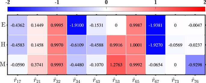
The value of element under each state reflects the regulation strength and regulation type (activated or inhibitory). The network topologies can be deduced by integrating these elements in three states.

Full size image

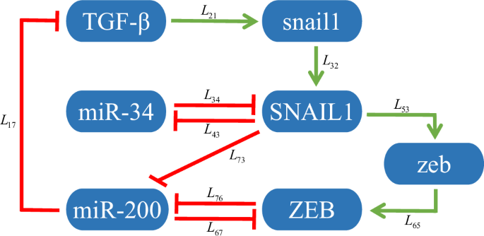
The regulation of node i by node j is denoted by L_ij, where i = 1,…, 7 represent TGF-β, snail1, SNAIL1, miR-34, zeb, ZEB, and miR-200, respectively.

Full size image

Compared to the true EMT network presented in Fig. 1, it is evident that two networks exhibit a remarkable similarity except that our approach fails to identify the regulation from ZEB to miR-34, i.e., ({hat{r}}_{46}(v)=0). The reason for the difference is that the actual regulation intensity ({r}_{46}^{0}(v)) is almost zero. While the values of r₄₆(v) calculated by Eqs. (2) and (3) under all resamplings satisfy the condition 0 within the 95% CI, resulting in ({hat{r}}_{46}(v)=0). Furthermore, the network topologies inferred in the EMT network using the redefined local response matrix are largely in agreement with experimental observations. Specifically, these inferred regulations are indeed present in the EMT network, as reported in studies^27,30,31. For instance, there are double-negative regulations between SNAIL1 and miR-34⁴², as well as between ZEB1 and miR-200⁴³. Additionally, miR-200 negatively regulates TGF-β⁴⁴, etc. In conclusion, it is remarkably accurate to utilize the redefined local response matrix to reveal the network topology, regardless of the perturbation degrees and perturbation distributions. This approach is especially advantageous in biology because there exist various noises and precise measurement is impossible in experiments.

Identifying critical information in EMT network

The redefined local response elements ({hat{r}}_{ij}(v)) offer qualitative insights into types and intensities of direct regulations between two nodes in each state. However, they are insufficient for quantitatively determining dominant regulations within each state or precisely identifying primary states associated with each regulation, solely based on whether ({hat{r}}_{ij}(v)) is non-zero. To overcome this limitation, we calculate the relative local response matrix (widetilde{{{boldsymbol{r}}}}(v)) under perturbation type I, which captures the relative importance of regulations in all states. Additionally, the relative WT local response matrix ({widetilde{{{boldsymbol{r}}}}}^{{{boldsymbol{0}}}}(v)) is also calculated to verify the feasibility of our approach, where ({widetilde{r}}_{ij}^{0}(v)={r}_{ij}^{0}(v)/{sum }_{v = 1}^{3}leftvert {{r}^{0}}_{ij}(v)rightvert).

To assess the accuracy of determining dominant regulations at each state or identifying primary states associated with specific regulations, i.e., characterize the difference between (widetilde{{{boldsymbol{r}}}}(v)) under perturbation type I and ({widetilde{{{boldsymbol{r}}}}}^{{{boldsymbol{0}}}}(v)), non-zero elements of ({widetilde{{{boldsymbol{r}}}}}^{{{boldsymbol{0}}}}(v)) and their corresponding elements of (widetilde{{{boldsymbol{r}}}}(v)) at E, H, and M states are depicted in Fig. 7A, B and C, respectively. By comparing the absolute value of ({widetilde{r}}_{ij}(v)) under perturbation type I or ({widetilde{r}}_{ij}^{0}(v)) with the threshold, 1/3, we can quantitatively identify primary cell states associated with specific regulations (Table 3), as well as determine dominant regulations at each cell state (Fig. 8). For each regulation, the darker the color at one state (the corresponding absolute value greater than the threshold 1/3), the more dominant in this state. Obviously, there is little difference between the information of (widetilde{{{boldsymbol{r}}}}(v)) under perturbation type I and ({widetilde{{{boldsymbol{r}}}}}^{{{boldsymbol{0}}}}(v)).

Each element within the boxes, distinguished by different colors, represents the relative regulation strength. The darker the color, the more important the corresponding regulation. The threshold for the relative strength is set at 1/3. Elements corresponding to unidentified regulations under perturbation type I are highlighted with orange boxes.

Full size image

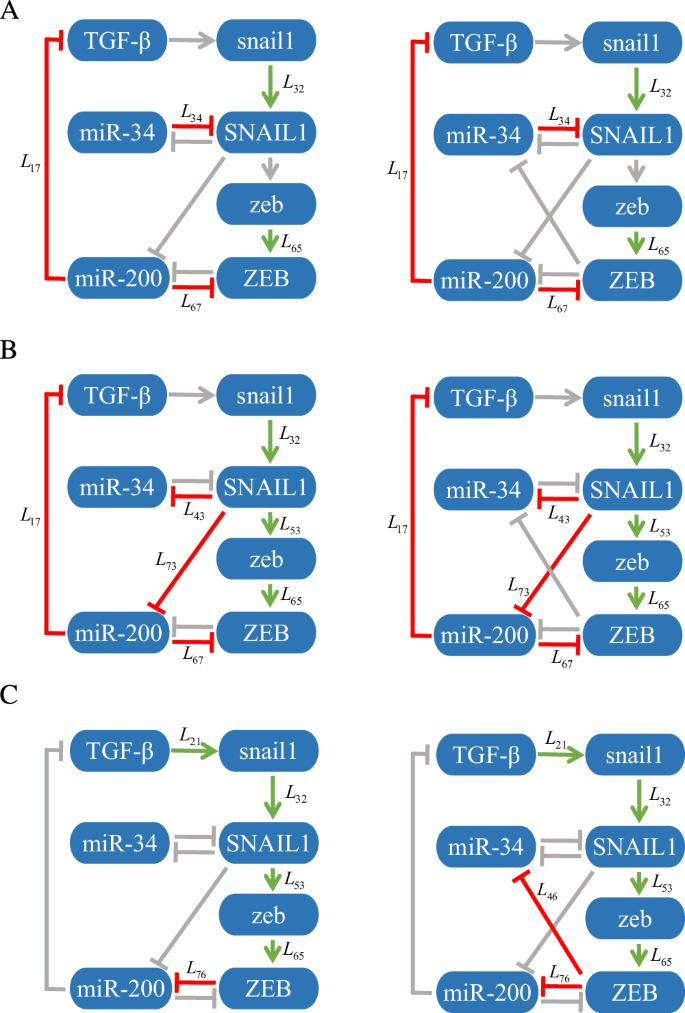
Using the relative local response matrix derived from perturbation type I and the WT relative local response matrix, as depicted in Fig. 7, the dominant regulations at each state have been identified and are indicated by green arrows and red bars. The non-critical regulations are represented as grey in each state.

Full size image

Specifically, to analyze (widetilde{{{boldsymbol{r}}}}(v)) under perturbation type I, we identify that the inhibitory regulations imposed by miR-200 on TGF-β and ZEB, i.e., L₁₇ and L₆₇, are dominant in both E and H states. The activation of snail1 by TGF-β, i.e., L₂₁, and the inhibition of miR-200 by ZEB, i.e., L₇₆, are critical in M state. The translation processes from snail1 to SNAIL1 and from zeb to ZEB, i.e., L₃₂ and L₆₅, are critical across all cell states because the relative regulation intensities are almost equal to the threshold 1/3. The inhibition of SNAIL1 by miR-34, i.e., L₃₄, dominates in E state. While the inhibitions of miR-34 and miR-200 by SNAIL1, i.e., L₄₃ and L₇₃, are critical in H state. The activation of zeb by SNAIL1, L₅₃, is dominant in H and M states. These results are shown in the second row of Table 3. Further, we identify the dominant regulations are L₁₇, L₃₂, L₃₄, L₆₅, and L₆₇ in E state, L₁₇, L₃₂, L₄₃, L₅₃, L₆₅, L₆₇, and L₇₃ in H state, and L₂₁, L₃₂, L₅₃, L₆₅, and L₇₆ in M state (the left panels of Fig. 8). These results are almost exactly consistent with those in²⁶, i.e., the critical regulations for common recognition are L₁₇, L₃₄, and L₆₇ in E state, and L₁₇, L₄₃, and L₆₇ in H state, and L₂₁, L₃₂, L₅₃, L₆₅, and L₇₆ in M state.

By analyzing ({widetilde{{{boldsymbol{r}}}}}^{{{boldsymbol{0}}}}(v)) (the third row of Table 3 and the right panels of Fig. 8), the inferred and true EMT networks at three cell states exhibit remarkable similarities with the exception of the identification of the regulation from ZEB to miR-34 i.e., L₄₆, which plays a dominant role in M state in the true network. Our approach fails to identify the critical states for this specific regulation because ({hat{r}}_{46}=0) in all these three states. Therefore, the dominant regulations identified at each state by our method, which is based on the relative local response matrix calculated from the perturbation data, aligns almost perfectly with the results obtained at the E, H, and M states using the WT relative local response matrix derived from the ODEs in²⁶. Evidently, the network inferences made by our method closely align with the true networks defined by ODEs, indicating good inference ability of the proposed approach.

Cell fate decision is a dynamic process based on mutual regulations between multiple molecules, and plays crucial role in the process of cell development. These intricate regulations form complex regulatory networks, serving as a fundamental tool in computational biology for exploring cell fate decisions. However, inferring the topologies of these gene regulatory networks remains a challenge due to their inherent complexity. In cell fate decisions, regulatory networks exhibit significant variations under distinct cell fates. As a result, if we are able to reconstruct gene regulatory networks which underlie these fate decisions, we can gain profound insights into the regulatory mechanisms behind various phenotypes. Consequently, we can precisely manipulate cells, guiding them into the desired specific state through quantitative control, which offers a practical solution for the treatment of various diseases, including cancer.

In this paper, we propose a general inference approach based on the data (experimental data, single-cell data, or stable steady states data obtained in silico analysis) before and after perturbations to accurately reconstruct gene regulatory networks, and further qualitatively identify network differences during cell fate decisions. Furthermore, our approach does not impose any limitations on the size of regulatory networks. Specifically, using the steady state data before and after perturbations for each cell fate, we first calculate the local response matrix based on Eqs. (2) and (3), where the value of element reflects regulation between molecules, and the larger the value, the stronger the regulation intensity. Then, based on statistical and differential analyses, i.e., the relative local response matrix from Eqs. (6) and (7), we can quantify network differences across all cell fates, namely identify critical regulations in each cell state and dominant cell states associated with specific regulations. Additionally, we have provided a verified method by comparing our results to the relative local response matrix calculated based on the ODEs of the system, referred to as the WT local response matrix. We use the EMT core network to verify the feasibility of our approach. By the differential analysis, critical regulations in each state and the main states associated with each regulation are accurately identified, which was consistent with some experimental observations.

Based on systematic perturbation, differential, and statistical analysis, a computational approach is developed to accurately infer gene regulatory network and identify network differences during cell fate decisions. The approach provides a general framework which can also be applied to infer regulatory systems, such as embryonic stem cell differentiation⁴⁵, cancer metastasis⁴⁶, hematopoietic cell differentiation⁴⁷, and other networks related to cell fate decisions^48,49. However, a limitation of the approach is that it cannot identify self-feedback loops, the direct regulation from one molecule to itself. Due to current limitation in experimental conditions, obtaining experimental data under perturbation conditions, such as single-cell data, is another challenge. Our future research will focus on how to infer gene regulatory networks with self-feedback loops by using experimental data under perturbations.

At the unperturbed stable steady state (bar{{{boldsymbol{x}}}}), the Jacobian matrix J is nonsingular and J_ii ≠ 0 (related to degradation and self-regulation). Based on the multivariate implicit function theorem for a small open neighborhood of the unperturbed stable steady state (bar{{{boldsymbol{x}}}}), we have

and

which means that the local response coefficient r_ij is related to the elements of Jacobian matrix at the unperturbed stable steady state. Consequently, we obtain

where ({{boldsymbol{X}}}={{rm{diag}}}(bar{{{boldsymbol{x}}}})) and diag(J) are nonsingular diagonal matrices composed by the unperturbed stable steady state vector and the diagonal elements of J, respectively.

Perturbation analysis of sensitive parameters

Generally, under a slight perturbation to sensitive parameter p_k, the stable steady state remains confined within a small open neighborhood of (bar{{{boldsymbol{x}}}}). Considering the derivative of f_i with respect to p_k, and using the multivariable chain rule, we have

Therefore,

where ({{boldsymbol{S}}}={left.(partial {f}_{i}/partial {p}_{k})rightvert }_{(bar{{{boldsymbol{x}}}};{{{boldsymbol{p}}}}_{{{boldsymbol{b}}}};{{{boldsymbol{p}}}}_{{{boldsymbol{c}}}})}), and P = diag(p_b) is a nonsingular diagonal matrix. According to diag(R⁻¹) = − diag(P⁻¹S⁻¹JX) = − P⁻¹S⁻¹diag(J)X, we find ({{boldsymbol{r}}}{{boldsymbol{R}}}=-{[{{rm{diag}}}({{{boldsymbol{R}}}}^{-1})]}^{-1}). Consequently, the local response matrix r can be solved only from the global response matrix R, i.e.,

which means that the local response matrix r can be directly inferred solely from R²¹. The calculation of R can be derived from the cell data gathered before and after the perturbations is applied to the sensitive parameter set, namely, Eq. (2). Therefore, we are able to compute r without needing detailed ODEs or exact parameter values.

Statistical analysis

To enhance the accuracy of inferring network topology, N distinct perturbation sets are utilized and thus N local response matrices can be calculated by Eqs. (2) and (3), i.e., r_l = (r_l,ij), l = 1,…, N. Specifically, a perturbed sensitive parameter set ({{{boldsymbol{p}}}}_{{{boldsymbol{s}}}}(l)=left({p}_{s,1}(l),cdots ,,{p}_{s,n}(l)right)), p_s,k(l) is randomly chosen from a uniform or normal distribution of p_k, k = 1,…,n. Consequently, we can derive the distribution of each local response coefficient and its corresponding 95% CI, which is delineated by the 2.5^th and 97.5^th percentiles of the distribution. This approach allows us to exclude insignificant regulations by evaluating whether their 95% CIs encompass zero, ultimately achieving sparse network. And for the nonzero regulations, we employ the mean of r_ij across the N sets to reflect the regulation strength from node j to node i. Then, the redefined local response matrix (hat{{{boldsymbol{r}}}}=({hat{r}}_{ij})) is used to represent the inferred network topology, where

Further, an error analysis is performed to determine the degree of accuracy between inferred network, (hat{{{boldsymbol{r}}}}), and true network, r⁰.

Differential analysis

Combining the concept of relative contributions of driving factors in ecosystem services⁵⁰, we employ the relative local response matrix, (widetilde{{{boldsymbol{r}}}}(v)), to quantitatively characterize the strength of a specific regulation across all cell fates, or to compare all regulations within a specific cell state. This approach enables us to identify the states where a particular regulation dominates, as well as the critical regulations which characterize each state. Specifically, the relative local response matrix (widetilde{{{boldsymbol{r}}}}(v)=({widetilde{r}}_{ij}(v))) is defined as follows

Next, we compare the absolute value of ({widetilde{r}}_{ij}(v)) with the threshold, 1/s, the regulation of node i by node j is significant in the v-th state when (leftvert {widetilde{r}}_{ij}(v)rightvert -1/s ,>, 0). Furthermore, the larger (leftvert {widetilde{r}}_{ij}(v)rightvert) is, the more significant the impact of the regulation on the v-th state becomes. Therefore, we can quantitatively represent the differences in the strength of each regulation across all cell fates, as well as evaluate the disparities of all regulations within a specific cell state.