General feature selection technique supporting sex-debiasing in chronic illness algorithms validated using wearable device data

Understanding sex differences in medical conditions is an important effort that has more recently gained broader attention within the United States and globally^1,2. In 2016, the National Institutes of Health (NIH) established a policy (NOT-OD-15-102; NIH) requiring “sex as a biological variable” (SABV)³ analysis in grant applications. While there has been an increase in the inclusion of females in clinical studies since The Revitalization Act of 1993, there has yet to be tangible increase in SABV analyses in the resulting publications within the US⁴. Outside of the US, the Sex and Gender Equity in Research (SAGER)⁵ guidelines were proposed by the European Association of Science Editors (EASE) Gender Policy Committee (GPC) in 2016 and were very recently adopted by the World Health Organization (WHO)^6,7 in 2023. These nascent guidelines have yet to result in a decisive shift towards consistent inclusion of SABV analyses in published research; however, it is known that prevalence rates between sexes significantly differ in many diseases and disorders. Specifically, there are differences in the prevalence of chronic metabolic disorders such as diabetes⁸, and cardiovascular conditions⁹ such as hypertension^10,11.

Diabetes and hypertension are global concerns. Using numbers from the US as an example, diabetes affects 14.7% of all adults in the United States, and nearly 5% of adults have an undiagnosed diabetic condition⁸. Females with diabetes have a greater relative risk of vascular disease for which the mechanisms for the increased risk are unknown, but may be linked to differences in care between females and males¹². In the US, hypertension prevalence in males and females is 51.7% and 42.8%, respectively¹¹, and often comorbid with diabetes, with 50-80% of individuals with type II diabetes also having a hypertension diagnosis¹³. While hypertension rates in non-diabetics are higher in males until the age of 64¹⁴, females with diabetes have higher incidence rates of hypertension¹⁵. Due to lacking SABV analyses and historically limited access to continuous monitoring technologies, symptoms and physiological variances across sexes have not been broadly explored.

New ways to measure and characterize human physiology across broad and diverse populations have recently become available through the emergence of wearable sensor devices (“wearables”). Wearables allow for long term monitoring of multiple modalities of data within an individual, allowing for more complex engineering of physiological features (e.g. daily rhythms^16,17, sleep composition¹⁸, menstrual cycles^19,20, etc.) than classical single time-point measurements (e.g. only having a single measurement taken during a clinical visit). Human biometrics continuously change for many reasons at many time scales, and the degree by which they vary is different for every person and, presumably, for each medical condition or combination of conditions. Effects on physiology have been measured in diabetes in short studies generally conducted while in the clinic or via participant surveys. In general, adults with diabetes have lower activity rates²¹, lower heart rate variability²², increased body temperature and heart rate^23,24, and general decreases in respiratory function²⁵ when compared to healthy individuals. There appear to be many causes for sex differences in the prevalence of diabetes²⁶ and hypertension^11,27, from genetics to behavior, and no definitive mechanism underlying these differences is known. Individuals with hypertension have been shown to have a higher finger skin temperature, respiratory rate, and resting heart rate during stressful activities²⁸.

Wearables have supported the emergence of health algorithms for classifying conditions (usually acute, as in COVID-19 onset^29,30,31,32), but to date, there is no systematic approach for ensuring that the features selected from these data are assessed for SABV. This is important because diseases manifest differently in different groups, and historically health algorithms developed using hospital records have had a tendency toward biased performance in men³³, with resulting lower precision and even harm being done in women^34,35 and minority populations^36,37. Here we present a strategy to support the systematic analysis of sex differences in the feature distributions for any longitudinal, physiological data set. This technique can also be used for the identification of features most relevant to classification of conditions given SABV, as would be used in developing a fair health algorithm. Using data sampled from the commercial wearable device, Oura Ring, we identify the heterogeneity between distributions across self-reported biological sex for different cohorts of individuals reporting either diabetes, hypertension, or both conditions comorbid. The latter provides support for consistency of findings across cohorts with similar conditions. Furthermore, we explore how the separability of features is dependent on the number of days of data that are included. Using these steps, we formed the main contribution of this work, a pipeline composed of two steps that rely on statistical techniques: identify the demographics that maximally separate cohorts of individuals; while holding those demographics constant for the groups with/without health conditions, identify the features that have minimal changes in effect size between the demographics while maximizing total separation of condition/no-condition. We hope that this process can be easily adopted, supports explainable algorithm development, and supports experimental planning for those intending to use SABV in their analyses.

We sought to develop and test a technique for identifying sex differences in feature effect sizes between individuals with and without conditions. We used diabetes and hypertension as examples due to their general prevalence in the US population as well as their increased prevalence in males compared to females, as this would likely contribute to male bias in algorithms developed on male-heavy data. Additionally, some individuals have only one condition or the other, where other individuals have both comorbid; this presents a natural experiment in which to test the consistency of these statistical approaches aimed at quantifying feature importance in different cohorts comprised of individuals who do or do not share diagnoses. The intention is to inform design considerations of feature selection pipelines that can be used to elucidate sex differences between cohorts that have the same reported condition. Here we present this intention using multi-dimensional wearable device data collected from individuals who reported having no condition, a condition, or comorbid conditions.

Theoretical consideration for separating cohorts

We imagined a chronic illness as having an effect on multiple physiological features. In a construct where these features are dimensions in a high-dimensional space, conditions can be identified as moving the centroid (e.g., median) of a cohort with no condition to the location of the demographic-matched cohort with target condition of interest – a vector of physiological difference through this high-dimensional physiological space. It follows that if different vectors of change are realized by different populations, then in aggregate, these vectors likely do not align perfectly, so that components from some vectors will then cancel others (Fig. 1). This will have the effects of reducing precision broadly (each populations’ unique vector has some projection distance onto the mean vector across populations), and also of biasing precision toward the most represented groups (whose vectors contribute more the mean). In the next section, we test this conceptual model by first creating cohort subgroups of each sex, age, and condition combination (e.g. older female with condition; or, younger male with no condition) from our data. Given a single feature (random variable), distributions can be compared to assess the null hypothesis that the distribution median from one population is the same as the distribution median from a different population.

A Cohort-Specific Medians. The medians of each no-condition cohort are shown as green dots. Each demographic cohort (sex: females in blue, males in red; age: < 40 yo more saturate color) has both a unique high-dimensional location of a condition (e.g. the small orange circles for each cohort are in different locations) as well as a unique manifestation of a condition (i.e. the vectors between no-condition medians to condition medians have different directions for different cohorts). Significance to a median with a condition may be easier to achieve even with lower power because effects are not averaged out as in (B). The pooled distribution from all individuals. The same vectors of change from (A) are added and move from the median of the large green circle to the pooled condition cohort. The average individual effects from each cohort no longer contribute significantly, because many different changes now cancel out.

Full size image

Clustering reveals a significant role of sex in determining feature similarity

In the TemPredict dataset³¹, participants reported chronic illnesses via a questionnaire. Of the original 63,153 participants, 12,387 reported a condition of interest (diabetes, hypertension, or both) or confirmed no condition and had at least one “usable” day of data (see Method, Physiological Data Information). Following the constraint that each individual had at least 28 days with data (minimum of 4 h while awake and 4 h while asleep, n = 10,844), cohorts were identified with diabetes but without hypertension (diabetes, “D,” 1.8%, n = 193), hypertension without diabetes (Hypertension, “H,” 18.6%, n = 2013), diabetes and hypertension (both, “B,” 2.3%, n = 252), or no chronic illnesses (confirmed no condition, “CNC,” n = 8386) from the provided list (Table 3). For females, 1.6% (n = 65) reported a diabetes diagnosis and 15% reported a diagnosis of hypertension without diabetes (n = 620). For males, 1.9% reported diabetes only (n = 128) and 20.8% reported hypertension without diabetes (n = 1393). Females represented around one-third of individuals who reported diabetes only (n = 65, 33.7%) or hypertension only (n = 620, 30.8%) and of those who reported diabetes (n = 117), less than half also presented with hypertension (n = 52, 44.4%). In males with diabetes (n = 328), 61% (n = 200) also reported having hypertension. From this we defined four cohorts each comprised of completely different individuals from the others: CNC, D, H, B (Fig. 2A).

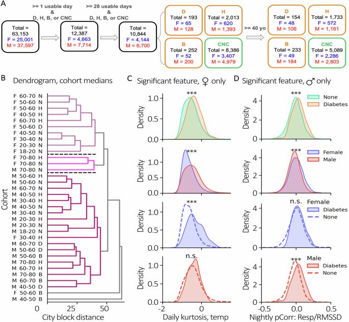
A Cohort filtering diagram. All individuals were first filtered by having at least 1 usable day of data as well as confirming one of CNC, H, D, or B. Then individuals were filtered as having at least 28 days of data. A subset was then selected for age over 40 years. Counts are shown at each step for the total cohort, females in blue, and males in red. B Features by Sex, Age, and Condition Dendrogram. Median sample of cohorts compared to each other with agglomerative clustering. Each color identifies a cluster that exceeds an average distance threshold from other clusters. Example features significant in exclusively females or males. Non-singleton clusters ordered top to bottom as 1, 2, and 3 and separated by black dashed lines. C Example feature, daily temperature kurtosis, with significant separability when considering condition or sex; however, when considering condition and sex, is only significant in females (blue) and not males (red). D Example feature, nightly pCorr respiratory rate (RR)/heart rate variability (RMSSD), that is statistically different in males but not females separated by the same condition. Two-sided, Mann-Whitney U, ***p < 0.001.

Full size image

We clustered cohorts on their features (see Methods, Physiological Data Information; Supplementary Fig. 1) and then assessed the relative value of chronic illness label, age, and sex on the explained variance of the resulting clusters. At a distance cutoff of 75% of max distance between centroids, the data revealed 3 non-singleton clusters (Fig. 2B). Using Chi-squared tests, we found a significant effect of sex (P < 0.001, Cramer’s V = 0.89), but not age (P = 0.84) or condition (P = 0.56) in accounting for similarities between non-singleton cohort clusters. In those clusters with sufficient data to allow for statistical comparisons with permutation tests, we found that cohorts were closest to their sex-matched and condition-matched neighbors in clusters 1 (P < 0.01) and 3 (P < 0.001) (Supplementary Fig. 2). We then lowered the distance cutoff to 65% to determine the effect that a moderate change in threshold had on the number of clusters identified. We observed 5 non-singleton clusters and reassessed the effects of each demographic category (Supplementary Fig. 3). There were significant effects of sex (P < 0.001, Cramer’s V = 0.95), age (P < 0.05, Cramer’s V = 0.667), and condition (P < 0.05, Cramer’s V = 0.665). Since the total distance between cohorts is dependent on a dissimilarity metric on the physiological features themselves, we investigated if these features consistently have the same effect size between sexes when comparing cohorts with and without conditions.

We scanned for features that separate “condition” and “no condition” subsets to understand if sex affected the effect sizes of those features. As an example, we found features that were significantly different between all individuals with no condition to all individuals with reported diabetes (P < 0.001) (Fig. 2C/D, top row) then filtered for features that showed a sex-effect when not accounting for condition status (P < 0.001) (Fig. 2C/D, second row). Figure 2C provides an example of a feature (Daily Kurtosis Temperature) that was significantly different between the cohort with no reported condition and the cohort with diabetes only in females; Fig. 2D shows a separate feature (Nightly partial correlation Respiratory Rate/RMSSD) that was significantly different only in males. We used this as an example of when the significance between a control cohort and condition cohort is driven primarily from a specific sex. Such features allow us to reject our null hypothesis that distribution changes in conditions are the same across populations (a list of all features that are differentially significant between sex can be found in Supplementary Fig. 1).

The effect sizes for physiological features that correlate to conditions are not consistent across reported sex

Now knowing that the same physiological feature might be differentially expressed in different sexes for the same condition, we calculated the extent to which all of our extracted features were affected by this phenomenon when comparing CNC to D and/or H cohorts. As the average age for D and H onset is above 40 years^38,39, and 86.2% of the condition cohorts consist of individuals above that age threshold, subsequent analyses were performed using data from participants older than 40 to reduce physiological heterogeneity across ages. We performed direct comparisons of Adjusted Common Language Effect Size (CLES, See Methods, Multiple Feature Separation by Condition and Sex) between males and females for the same features and visualized them with a scatterplot. The comparisons were determined by which test cohort was used and which condition cohort was used (Fig. 3). If both sexes had the same Adjusted CLES for a feature, then its point would fall along the identity line (x = y) in the plot. If the feature separated females better, then its point would fall below the identity line, and for better separation in males the point would fall above the identity line.

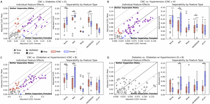
Left Panels. Analyses of differences in effect size separation between control condition and test condition for each sex for all features. A CNC cohort compared to D cohort. B CNC cohort compared to H cohort. C CNC cohort compared to B cohort. D D cohort compared to H cohort. The solid identity line is where the effect size for a feature is equal in females and males. Parallel dotted lines below the identity line reflect a 5% increment increase in feature separability in females, and dotted lines above the identity line reflect a 5% increase in feature separability in males. Gray, blue, red, and purple markers indicate features that are significant in neither sex, females only, males only, or both sexes, respectively. Right Panels. Separability of features by feature type within and across sex. Red and blue boxplots are comprised of the effect sizes from features that are significant in males and females, respectively. Each individual boxplot was evaluated with a one-sided Wilcoxon signed rank test to evaluate if the aggregate effect size of significant features is equal than 0, with significance annotated directly above the boxplots (*p < 0.05, **p < 0.01, ***p < 0.001). For each feature type, a paired, two-sided Wilcoxon signed rank test was used to evaluate if the effect sizes from significant features are equal between males and females (*p < 0.05, **p < 0.01, ***p < 0.001)

Full size image

In comparing the feature distributions from the CNC cohort to those in the diabetes cohort (CNC vs. D), 31 features were significantly different in both females and males, 10 features were only significantly different in males, and 5 features were only significantly different in females (Fig. 3A, left). While there were only 5 features that had at least a 5% increase in cohort separability for males compared to females, there were 14 that had at least a 5% increase in females compared to males. Of those, 12 of the 14 features were derived from either temperature or activity data. We found that, in aggregate, there were larger effect sizes in temperature- (P < 0.05) and activity-derived (P < 0.01) features for females; in males, there were larger effect sizes in cardiac-derived features (P < 0.05) (Fig. 3A, right; Visualization of significant features found in Supplementary Fig. 1, CNC vs. D).

In the CNC vs. hypertension comparison (CNC vs. H), 53 features were significantly different in both females and males, 8 features were only significantly different in males, and 7 features were only significantly different in females (Fig. 3B, left). Only 2 features had at least a 5% increase in separating females than males, which were both temperature-derived. We found that activity- and cardiac-derived features were better at separating females compared to males (P < 0.05) (Fig. 3B, right; Visualization of all features and their relative effect sizes are found in Supplementary Fig. 1, CNC vs. H).

In the CNC vs. both comparison (CNC vs. B), there were 41 features significant in both sexes, 16 features that were only significantly different in males and 2 features that were only significantly different in females (Fig. 3C; Supplementary Fig. 1, CNC vs. B). Several activity-derived features increased from having around a 5% improvement in separability in females compared to males for either exclusive diabetes or hypertension, to having around a 10–15% increase in separability in the B cohort. There were larger effect sizes in both temperature- and activity-derived features in females (P < 0.001). Although cardiac-derived features were more separable for males in D and females in H, the sex-based separability for cardiac-derived features for B was not significantly greater in either sex (Fig. 3C, right).

To assess whether there is consistency in the findings across cohorts, we compared the differences in the D cohort to those from the B cohort. In our dataset, 60% of the individuals with diabetes have hypertension, whereas only 11.9% of the individuals with hypertension have diabetes. We wanted to investigate the separability found from this statistical technique when comparing two similar cohorts, thus we chose diabetic individuals as a control and diabetic individuals with hypertension as a test. Since diabetes had larger effect sizes overall, we anticipated that there should be a diminished ability to separate D from B. We observed that none of the features were significant when attempting to separate the groups (Fig. 3D), confirming that the separations found in D are also found in B. However, there was significantly better separation in females from activity-derived (P < 0.001) and pCorr (P < 0.05) features compared to males (Fig. 3D, right).

The amount of data sampled from each individual does not necessarily lead to similar greater statistical separation in both females and males

Up to this point we had only used the median of all data from each individual with at least 28 days to create our cohorts. Multiple samples from the same individual were median-aggregated to maintain the assumption of independent and identically distributed (IID) data for statistical comparisons. Given that these data accrued as time series, this raises the question as to whether the differences we observed were stable over time, and/or whether there is a consistent amount of data from each individual that reveals these effects reliably. As the total amount of data collected per individual may have an effect on the Adjusted CLES, we evaluated how effect size changes with the amount of data accumulated to understand the minimum amount of data needed per person to create a representative distribution prior to considering the median (Fig. 4).

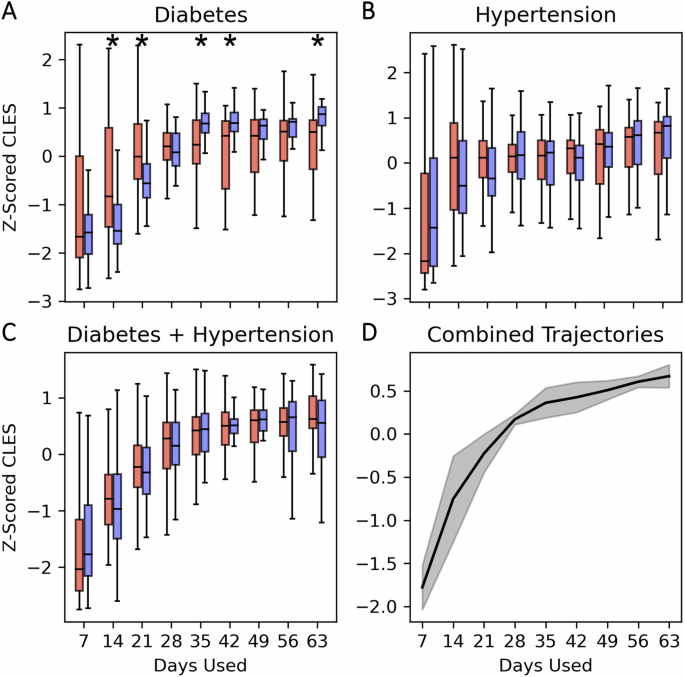
Each boxplot contains the z-scored Adjusted CLES for males (red) and females (blue) when using the median of different numbers of days used per individual. A Diabetes, B hypertension, and C diabetes with hypertension. D Median curve of the median Z-scored CLES for each sex/condition trajectory. Shaded region is the standard deviation of the median trajectories. Male and female boxplots are compared with two-sided Wilcoxon signed rank tests to evaluate if they have their distributions come from the same median (* indicates p < 0.05). Significant differences between females and males by number of days included in analyses were only found in the cohorts with Diabetes alone (A).

Full size image

In D, we observed that the Adjusted CLES in both sexes reached stable effect sizes at around 28 days of data (Fig. 4A). The effect size change based on the number of days used had the same increasing behavior for both sexes; however, males had greater relative effect size at 14 and 21 days used (P < 0.05). Alternatively, females had greater relative effect sizes at 35, 42, and 63 days used (P < 0.05).

In hypertension (both alone and comorbid with diabetes), we observed that the effect size also began to taper off at around 28 days for both sexes (Fig. 4B, C). There were no significant relative differences found between both sexes in how effect size changes as the amount of data used for each individual increases.

Overall, we observed a trend where CLES between CNC and condition cohorts in both sexes tended to increase in all conditions as more days of data were aggregated per individual until around 28 days. After 28 days, the CLES appeared to stabilize and the variance around the CLES likewise reduced and stabilized (Fig. 4D).

Here we confirmed that the same condition can lead to heterogeneous observed physiological effects between females and males when using features derived from longitudinal wearable device data. We further confirmed that sex was a leading contributor to automated attempts to cluster individuals based on their physiology, above both age and condition. This supports the need for SABV analysis to support appropriate algorithm development from continuous data. We developed a statistical approach to systematically quantify the extent to which any set of features differs in a given condition as a function of sex. Applying this technique we found that different features were indeed affected by sex in different chronic conditions of hypertension and diabetes. We confirmed that these differences were likely not false discoveries by comparing a cohort with both conditions to the cohort with one condition most likely to develop eventual comorbidities with the other (i.e. diabetes to hypertension), and found that these cohorts overlapped substantially in the sex effects of features. This is consistent with the hypothesis that similar physiological patterns of change should persist from individuals with diabetes across those who also develop hypertension as a comorbidity. By using a novel arrangement of established statistical comparisons in the emerging context of longitudinal and continuous multimodal data, we demonstrate the potential for generating two types of novel insight: 1) architectural insights akin to feature engineering, but here for feature selection to constrain the possible paths of tree-like ML models in order to systematically reduce algorithm bias against women; 2) insights to guide the appropriate selection or engineering of sensors so that studies on physiology can quantify possible bias from sex differences of information per sensor modality.

Many condition classifiers built on physiological data, as in those gathered by wearables, work by assuming that disease processes manifest as a movement away from the centroid of the physiological space defined by the control class^{40,41,42,43,44,45}. In our cluster analysis we found that the distance between cohorts associated with conditions was actually not significant compared to the distance associated with sex. It was only when lowering the threshold did the effects of age and condition become significant. For this reason, first separating groups by sex allows for more precise detection of these smaller movements than would be possible when measuring against all clusters lumped together as one. In fact, we found that the direction of the condition-associated movements was different between the groups, which is why failure to separate by sex and age may lead to averaging of opposing directions, thus making appropriate detection systems more difficult to build, or inappropriate for one group over another.

The WHO lists the social and economic environment, the physical environment, and a person’s individual characteristics (such as sex) and behaviors as determinants of health⁴⁶. Standards vary for each nation, but the need to report and include analyses by sex have been recognized globally^3,5,6,7. These factors just listed will change by region and nation. As SAGER and related standards are adopted, local validations will likely be needed. Conceptually these separate efforts are unified in that the comparisons being made within each such effort can be considered as high-dimensional feature spaces that are often embedded into categorical features for data science (DS) and machine learning (ML) tasks. Specifically, the genetic, physiological, behavioral, social, and environmental differences that exist between females and males are (lossily) transformed into a variable that can be easily stored as a value in a database row: Sex. In the context of the features we derive from the Oura Ring physiological data streams, we see that the underlying biological system (female/male physiology) explains more similarity between cohorts than both age and conditions. For example, if conditions (or lack thereof) explained the most variance in the data, then it is likely that individual clusters would form around them regardless of sex. However, we see that this kind of clustering only appears once we condition on the sex of the cohort. The scope of this work was to statistically test the extent to which sex differences in features could be cleanly separated. We found that there were many heterogeneous relationships between features by sex. This is consistent with the concern that algorithms trained only using sex as a label would be unlikely to correctly identify the complexity of these differences. Instead, mapping the feature importance separately for each group of concern (here, sex) is likely to be a more efficient means of ensuring that the most salient features for each group and condition are appropriately used for algorithms trained to identify that group and condition. We show that including a label such as sex does not alone account for the many non-linear changes that result from sex differences in feature engineering. We believe this approach can reasonably be applied to the comparison of further race/ethnicity groups as well, but such analyses are beyond the scope of this manuscript. Iterations of experiments will be needed to identify which features and which data sources are the most reliably useful for specific populations and conditions.

We first show that there is a significant effect of sex in how cohorts cluster in our high-dimensional physiological feature space. This confirmed our hypothesis that there are gross differences between cohorts, but this did not highlight which features contribute greater separation between sex. To move away from large feature spaces and into singular comparisons, we then visualize how physiological features can have different effect sizes as well as different null hypothesis rejections within the same condition between females and males. Interestingly, we observe an inverse relationship between how many features are “biased” toward females or males and the population-level prevalence of those conditions (diabetes⁸, hypertension¹⁰). We point this out not to indicate any sort of statistical relationship, but rather to highlight the potential risks of either not accounting for potential sex differences in physiological data or by believing a statistical model developed in one sex should be generalizable to the physiological data in a different sex. Furthermore, we separate the features by type to show how selecting certain sensors for a longitudinal study may have effects on what level of statistical separations are found in females and males. Greater effect sizes across multiple data streams for the same sex give a strong indication that there may be multiple ways that different sexes manifest the same condition, or that the expected physiological covariates with a given condition may in fact covary in different ways across sexes. For example, different study considerations may need to be made in instances where females have greater effect sizes in features derived from temperature and activity, and males have greater effect sizes in features derived from cardiac or respiratory features. This would indicate that the kind of wearable device or set of sensors used to infer that condition would have an effect on cohort separability in a study. Out of 14 wearable devices reviewed by Vijayan and Connolly⁴⁷, 2021, only 1 had a temperature sensor while 8 had the ability to estimate heart rate. In the example just given, derived from our observations here, this might well bias detection in favor of males due to the lack of female-appropriate temperature sensors. As mobile health technologies become more widespread and the longitudinal data generated from them become used in predictive health applications, it is important to consider that feature streams beyond estimated heart rate may increase the performance of inference models for specific sexes.

Furthermore, we show that there are sex-specific effects related to how the subset of samples from an individual’s total time monitored may lead to effect-size increases for longitudinal physiological features. While each individual was monitored for longer periods of time, we use an increasing set of samples to control for within-individual variability, observing a plateauing effect of time on separability after 28 days. This suggests that 28 days of data may be a reliable minimum amount of data from which to extract sex differences associated with conditions from longitudinal physiological measurements, and, more specifically, may be a recommended minimum number of days needed for wearable devices feature selection. Though there is a general trend where more days of measurement leads to greater effect size, separability in diabetes is disproportionately increased in males when using fewer days of data, and then disproportionately increased in females when using more days of data.

Put plainly, we call attention to the differing statistical separability of the same physiological features across sex to show that even if females and males may have the same condition, those conditions may present in different ways due to a multitude of factors. This point highlights several limitations of our study. First, the data gathered is not from a certified research device, but a consumer device. While this may introduce noise and uncertainty into the data (we don’t know – a lack of certification does not imply reduced signal quality), it also allows us to monitor large numbers of individuals for extended periods of time at no added cost, as devices were used by the participants already. Second, the survey information used to identify cohorts with a condition (or lack thereof) does not specify if each individual presented with the condition and/or received treatment during the study period, nor does it indicate time since diagnosis. This can lead to concept drift – the length of time in which an individual has a condition generally increases the accrual of deleterious effects. These effects can manifest as variance within the physiological features extracted, and we cannot assess the contributions of change over time within individuals in this work; for this reason, we make no attempt to optimize a classification task. In terms of cohort bias, it is likely that the owners of the Oura Ring were likely wealthier with higher levels of education than the average population. As no information regarding participant socioeconomic status was collected, we were unable to account for its effect. The dates over which data were gathered includes the start of the COVID-19 pandemic as well as its eventual height (January – November, 2020). Since the pandemic dramatically changed daily behavior globally, we cannot account for this behavioral variability compared to pre-pandemic periods. Despite this unexplained variance, we found consistent effects of change across cohorts with the same condition label, and propose that our methods can assist in quantifying and localizing sex differences in any longitudinal data set. This information might be used to predict bias, and to shape design choices in algorithm design and in future studies aimed at closing our sex-biased medical knowledge gap.

With females continuing to be underrepresented in research and clinical trials^4,48, it is important to ameliorate cohort bias in the younger field of mobile health to ensure equitable longitudinal condition monitoring. Sex is not a categorical variable to be accounted for, but rather a model to evaluate differences in health and manifestation of disease. Furthermore, wearable data is merely an example dataset that can be used for these analyses. We believe that iterative statistical quantification of physiological differences using continuously measured digital biomarkers should improve the interpretability of any model that aims to evaluate the properties of sex-specific dynamics of health and the sex-specific manifestation of conditions.

We observe that effect sizes for the same physiological features as well as the value of specific feature/sensor types are significantly affected by sex. The extent to which sex affects how physiological manifestations change for a given condition is an underexplored space. While sex bias has been an issue in clinical trials and cohort selection both historically and currently, we can improve upon this by using SABV analysis in the emerging field of mobile health algorithms. We propose that statistical approaches that are designed to highlight such sex differences can lead to better interpretations of how conditions uniquely manifest in such disparate physiological systems, how sensor choice might affect our ability to detect these differences, and how future work can be designed to target and make use of differences to reduce algorithm sex bias.

Wearable device and questionnaire data collection

All data were part of the TemPredict Study in which data was collected from January to November, 2020^20,49. The dataset includes physiological data generated using the wearable device Oura Ring (Oura Health Oy, Oulu, Finland), as well as survey data such as self-reported sex, age, race, and ethnicity. All participants wore the Oura Ring Gen2 (Oura Health Oy, Oulu, Finland), a commercial wireless device worn on the finger that contains 3 separate sensors: negative coefficient (NTC) thermistor (resolution of 0.07 °C) to detect distal body temperature (DBT), a tri-axial accelerometer to measure activity (metabolic equivalents, MET, resolution of 60 s), and a photoplethysmography (PPG) sensor (signal sampled at 250 Hz) that measures heart rate (HR), heart rate variability as measured by the root mean square of successive inter-beat intervals of the PPG (RMSSD), and respiratory rate (RR)³¹. All data was wirelessly synced via bluetooth from the ring to the user’s smartphone when the Oura App was in use. Data from the app was then sent by the app to Oura’s cloud architecture, from which we received a one-time data push from their secure Amazon storage (S3) to our S3 cloud storage located on San Diego Supercomputer (SDSC) infrastructure.

In addition to the wearable data, participants had the option to answer a questionnaire related to chronic illness via the app. Demographic questionnaire data included approximate age in years (“What is your age?”), sex (“What is your biological sex?”), ethnicity (“Are you of Hispanic or Latino Origin?”), race (Options: African American / Black, Asian, Caucasian / White, Middle Eastern, Native American / Native Alaskan, Native Hawaiian / Other Pacific Islander, South Asian, Other Ethnicity [optional text]), and country of residence (“Select the country in which you are currently residing”). A question related to illness asked “Have you ever been told by a healthcare professional that you have, or have been treated for, any of the following conditions (in the past or currently)?” with options “diabetes (not including pre-diabetes),” “High blood pressure or hypertension,” and “None of these”. The “None of these” options indicated the participant has not had any of the following conditions: high blood pressure or hypertension, diabetes, coronary artery disease or angina, a heart attack, congestive heart failure, stroke or transient ischemic attack, atrial fibrillation, sleep apnea, COPD (emphysema, chronic bronchitis), asthma requiring regular inhaler use, cancer, anemia or other blood disorder, immunodeficiency including HIV, or other respiratory issues.

Ethics approval and consent to participate

The University of California San Francisco (UCSF) Institutional Review Board (IRB, IRB# 20-30408) and the U.S. Department of Defense (DOD) Human Research Protections Office (HRPO, HRPO# E01877.1a) approved of all study activities, and all research was performed in accordance with relevant guidelines and regulations and the Declaration of Helsinki. All participants provided informed electronic consent. We did not compensate participants for participation.

Physiological data information

Features were derived from 5 wearable data modalities (temperature, activity as metabolic equivalents (MET), heart rate (HR), heart rate variability (RMSSD), and respiratory rate (RR)) collected for all individuals that had at least 28 “usable” days (Table 1) with asleep and/or awake state data (Table 2). In total, 82 features were extracted from the 5 modalities, and are listed in Supplementary Fig. 1. A “usable” day is defined as a day that has at least 4 h of non-missing temperature data during awake state and at least 4 h of non-missing temperature data during asleep state. The awake/sleep states were assigned from the longest daily sleep window identified by Oura’s sleep staging algorithm. The data after removing missing values was not required to be contiguous. Features derived from each valid awake or asleep state include mean, standard deviation, skew, kurtosis, and mean of the first derivative. An additional feature for each pair of data streams was generated to capture relationships between the modalities using partial correlation (pCorr). The pCorr features were calculated by first fitting linear models of the confounding variables to the two variables of interest. Then, the residuals of the two variables of interest were compared for linear correlation. If the two signals were uneven due to missingness in one datastream but not in the other, the pCorr calculation was only performed on pairs of datastream data if non-missing values existed in both streams. Therefore, the pCorr calculation represents the minimum set of paired data across all datastreams with non-missing data. Only temperature and activity (Met) are collected during awake states due to the sensitivity of PPG to motion artifacts, which negatively impacts the confidence estimation of RR, HR, and RMSSD.

Cohort selection

Overall, 63,153 owners of an Oura Ring volunteered their wearable data for the TemPredict study^20,49. Of those participants, 12,387 had at least one “usable” day, as defined above, and reported either no conditions in the provided list or a diagnosis of diabetes, hypertension, or both (Fig. 2A). To account for variability across days sampled, we further filtered to individuals with at least 28 “usable” days of data (total n = 10,844, female n = 4144, male n = 6700). As the average age of onset for both diabetes (US average age of onset 47–52, depending on race/ethnicity³⁸) and hypertension (mean diagnosis age = 46³⁹) is over the age of 40, a sub cohort was created limiting participants to those 40 years of age and older (total n = 7209 total, female n = 2,955, and male n = 4254). Demographics for both the all ages and greater than 40 years of age cohorts are reported in Table 3.

Features by sex, age, and condition dendrogram

Three demographic labels were used to generate cohorts: reported sex, age bin, and condition. Reported sex is whether someone identified themselves as “female” or “male” in the survey. Age bins are roughly based on decades (e.g. 20-30 years, 30-40 years, etc.) with the exception of 18-20 years. The oldest age group is 70-80 years. The condition is one of “CNC” (confirmed no condition), “D” (diabetes), “H” (hypertension), and “B” (both diabetes and hypertension). Cohorts therefore became groups of sex_age-bin_condition, where a cohort is only created if there are at least 10 individuals that fit the criteria and have at least 28 days of data. The median value of each physiological feature for a cohort was calculated to create a sample that represents the high-dimensional centroid sample/individual of a cohort. After z-scoring each feature across the cohorts, the Python library scipy.cluster.hierarchy was used with city-block (“Manhattan”) distance and average linkage to cluster the cohort medians. A cluster was denoted with a unique color if its upper most level and all descendants are at least 75% of the maximum distance to any other cluster in the data. Chi-square tests were performed with clusters as groups and demographic labels as conditions. Each Chi-square test held the cluster groups constant while changing the frequencies depending on the demographics for (exclusively) sex, age, and condition across clusters. Cramer’s V was calculated from the Chi-square test statistic for the tests on sex, age, and condition.

Within-cluster physiological centroid distance compared to demographic distance

For each demographic cohort (e.g. female_70-80_D), a physiological centroid was calculated as the location in the high-dimensional feature space generated from the median feature value along each of the feature dimensions (i.e. median nightly HR, median nightly Temperature, etc.). Physiological centroid distance is the City-Block/Manhattan distance between cohort medians to determine which cohort was closest in the high-dimensional feature space. We use the centroid distance to determine each cohort’s nearest neighbor.

Between each demographic cohort, a demographic distance was created between each sex_age-bin_condition. If two cohort descriptions had different sex, total demographic distance increased by 3 (to ensure the already observed large effect of sex does not incorrectly place different-sex groups as adjacent). If two cohort descriptions had different age-bins, total demographic distance increased by 1 for each ordinal age-bin apart the cohorts were (e.g. 20-30 and 30-40 would be a distance of 1, while 30-40 and 60-70 would be a distance of 3). If two cohort descriptions had any two different conditions between “CNC,” “D,” “H,” or “B,” the demographic distance increased by 1. As an example of demographic distance in practice, the cohort of females aged 20-30 with confirmed no condition (female_20-30_CNC) and females aged 40-50 with diabetes (female_40-50_D) would have a distance of 3: 2 for each age bin of separation (20-30 vs 40-50), and 1 for the condition difference (CNC vs D). As such, the minimum demographic distance is 1 (e.g. male_20-30_CNC vs. male_30-40_CNC) and a maximum demographic distance of 9 (e.g. male_20-30_CNC vs. female_70-80_D).

Using both the demographic and physiological centroid distances, we determined pairwise proximity across all cohort centroids. For example, if we identified two cohorts that were nearest neighbors in the high-dimensional physiological space and the demographic distance between them was 1 (i.e. there is only one demographic label of separation), then we identify a pair of cohorts where a demographic nearest neighbor is also a physiological nearest neighbor (Note: If Cohort 2 is the closest neighbor to Cohort 1, it does not necessarily mean that Cohort 1 is the closest neighbor to Cohort 2).

We then constructed null hypothesis distributions to find the likelihood of observing that a demographic neighbor is also a physiological neighbor compared to random chance. For each cluster from the dendrogram, we separated the demographic labels of the constituent demographic cohorts from the physiological data. We performed 1000 iterations of random shuffles on each column containing physiological data from the individuals that comprise a demographic cohort(i.e. Night Mean HR for one subject would likely move to another subject after shuffling, but would not leave the Night Mean HR column) and then appended it back to the demographic labels, thus divorcing the meaning of physiological distance from demographic distance. The null hypothesis was rejected if the frequency of observing that a demographic nearest neighbor was also a physiological nearest neighbor within a cluster was at least in the 95th percentile of frequencies from the 1000 shuffles.

Example features significant in exclusively females or males

Data from all individuals was used for the comparison of physiological features. Each individual was represented as the median of their days to maintain IID assumptions. Mann-Whitney U tests were used to compare the medians of the physiological features across the four comparisons: 1) all individuals with no reported condition and all individuals with reported diabetes, 2) all females and all males, 3) all females with no reported condition and all females with reported diabetes, and 4) all males with no reported condition and all males with reported diabetes.

The features were post-hoc selected from a set of physiological features where there is a significant effect across conditions as well as a significant effect across sexes, but no significant effect across conditions when accounting for sex in one of the sexes.

Multiple feature separation by condition and sex

Mann-Whitney U tests were performed for the comparison between all physiological features when accounting for reported sex. The common language effect size (CLES) was used to calculate the likelihood that the value of a physiological feature from one distribution is greater than the value of the same physiological feature from another distribution⁵⁰. We used the non-parametric, brute-force method of the calculation to perform exhaustive pairwise comparisons between all samples in the distributions. We use CLES because regardless of the size of the cohorts, the measured effect sizes for significant results are less affected with this non-parametric method.

For the example of two perfectly overlapping distributions, the CLES would be 0.5 since it is a 50/50 chance that the samples from one distribution are greater than the samples from another distribution. Therefore, CLES results less than or greater than 0.5 for significant results indicate if the control distribution has a median less than or greater than the test distribution, respectively. We convert CLES to an Adjusted CLES to directly compare the effect sizes independent of direction:

For example, a CLES of 0.4 and 0.6 would both be 0.1 to more easily be compared in the scatterplot, since we are more interested in how much each physiological feature separates the cohorts regardless of direction of effect.

The workflow described within the above sections is summarized in Fig. 5. Briefly, after initial feature engineering, demographic and condition labels are used to separate subjects into cohorts. The pairwise distances between the medians of the cohorts are subsequently calculated, to identify a number of demographics, d, with the highest physiological distances. Using those d demographics, the within cohort significance and effect sizes between condition status (e.g. D, H, B, CNC) is calculated. Lastly, a final number of features, f, are selected based on the union of the highest individual effect size and lowest differential effect size (magnitude difference of effect size between demographics of interest, e.g. female vs. male).

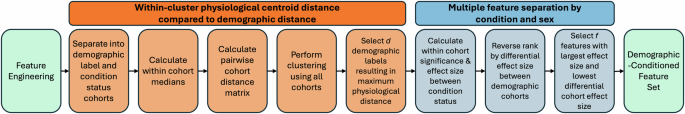
First, identify within-cluster physiological centroid distance and select the d demographic labels that have the largest physiological distance. Second, select f features that best separate conditions (effect size) and vary least between demographic labels (differential effect size).

Full size image

Separability of features by feature type within and across sex

We labeled the features derived from the Oura Ring as specific “types” depending on which signal they were derived from or if they are interactions of features. We make the decision to group HR and RMSSD together since they are both calculated from the same interbeat-interval data and have a strong functional relationship to each other at the 5-min scale⁵¹. Additionally, we created a unique feature group comprised of partial correlations between each pair of data streams (pCorr). Partial correlation for each pair of features is the same as the Pearson correlation between the same pair of features when accounting for the effects/residuals of the other features. It attempts to find independent linear associations between features whereas Pearson correlation does not attempt to find independence.

Each feature type for both females and males is first evaluated with a one-sided, one-sample Wilcoxon signed-rank test to evaluate if its Adjusted CLES has a non-zero median. A paired, two-sided Wilcoxon signed-rank test was used to evaluate if there was a difference in median Adjusted CLES between females and males when observing the same feature type. Significance of both tests was evaluated at ɑ = 0.05.

Effects of increasing number of days used in analysis

From the same set of individuals with at least 28 days of data, we iteratively took increasing numbers of days prior to calculating the median sample for each individual in 7-day increments. Individuals were dropped from analysis if they did not have the amount of days needed at a specific increment. For each number of days used and for each feature, the Adjusted CLES was calculated between the group with no reported conditions and the group that reported a condition, with females and males separated. Each feature was z-scored relative to itself across the number of days sampled in both females and men. A paired, two-sided Wilcoxon signed-rank test was used to then determine if the relative increase in Adjusted CLES as a function of number of days used was different between sexes. We use the Benjamini-Hochberg procedure to control the false discovery rate at ɑ = 0.05.