Geographical origin discrimination of Chenpi using machine learning and enhanced mid-level data fusion

Citri Reticulatae Pericarpium, commonly known as “Chenpi” in Chinese, which originates from the dry peel of Citrus reticulata Blanco or its cultivars. Chenpi’s medicinal history dates back to its first mention in the Shen Nong Ben Cao Jing in the period of Qin and Han Dynasty¹. It is a drug-eating homogeneous medicinal material, and clinically used to treat nausea, vomiting, indigestion, anepithymia, diarrhea, cough, expectoration, and so on². Chenpi is mainly produced in the provinces of Guangdong, Jiangxi, Sichuan, Fujian, and Zhejiang in China. The Chinese Pharmacoloeia (Chinese Pharmacopoeia Commission, 2020) records four varieties: Guang Chenpi, Chuan Chenpi, Zhe Chenpi, Pericarpium Citri Reticulatae and Jian Chenpi. Among these, Guangchenpi makes up 70% of the total Chenpi production³. The Guangchenpi cultivated in Xinhui district of Guangdong province are regarded to be the most authentic and to have special flavor and taste⁴, meriting a premium price compared with Chenpi originating from other cultivars⁵. However, the morphological similarity between Guangchenpi and other Chenpi types has led to frequent adulteration, as lower-quality Chenpi is misrepresented as Guangchenpi to increase profits⁶. This issue underscores the necessity of developing an effective, rapid, and reliable method for authenticate Chenpi’s geographical origin, ensuring quality assurance and consumer trust.

Phytochemical studies have identified various components in Chenpi, such as volatile oils, flavonoids, alkaloids, microelements, vitamins, pectin, and polysaccharide. In previous studies, several kinds of strategies have been proposed for discriminating Chenpi from Guangchenpi. The most commonly reported strategy is to identify the influential markers of flavonoids^7,8,9,10, and volatile compounds^4,6,11,12. Table 1 provides a summary of the above mentioned influential markers that applied to discriminate Chenpi and Guangchenpi. While these methods are show effectiveness in differentiation, they often face limitations. The lack of uniform criteria for compound selection can lead to discrepancies in findings, as different studies may identify distinct compounds for the same purpose. This inconsistency poses challenges in cross-study comparisons, impedes the development of universally applicable chemical markers, and limits the reproducibility of results. Furthermore, additional methods have been reported, such as the identification of different kinds of Chenpi using deoxyribonucleic acid (DNA) barcoding¹³. While this approach offers excellent discrimination accuracy, it relies on comprehensive DNA databases and has high requirements for sample quality¹⁴. Therefore, despite these advancements, there is still an obvious need to develop a method with good universality that can rapidly and accurately identify the geographical origin of Chenpi.

Data fusion is an emerging analytical method, enabling more useful information and satisfactory analytical results to be obtained¹⁵. In general, data fusion strategies can be divided into low-level, mid-level, and high-level approaches¹⁶. In low-level data fusion, data obtained from different sources are directly concatenated to establish an analytical model. In mid-level data fusion, the important features are independently extracted from each dataset and then combined to establish an analytical model. High-level data fusion calculates the analytical results separately on the basis of each dataset, and then combines these results to obtain the final analytical output¹⁷. When combined with data from different analytical techniques, data fusion has proven effective in enhancing food authenticity detection. For example, low-level data fusion has been successfully applied to classify different kinds of olive oils¹⁸ and different species of fish¹⁹. Similarly, mid-level data fusion has been applied to classify beer²⁰ and to identify the geographical origin and production methods of salmon²¹. In contrast, high-level data fusion is less commonly used in the field of food authenticity, primarily due to its increased complexity compared to low-level and mid-level data fusion²². In the analysis of complex samples, the original analytical data consists of a large number of variables, many of which include redundant information that is irrelevant to the sample. This redundancy can complicate data analysis and hinder the accuracy of results, emphasizing the need for important information extraction²³. Several studies have demonstrated that better analytical results can be obtained by mid-level data fusion, which utilizes a small number of important variables²⁴. Although data fusion strategies have been successfully applied in many fields, to the best of our knowledge, only a recent study has reported using low-level data fusion to discriminate between Chenpi and Guangchenpi²⁵. This highlights the need for further exploration of data fusion techniques, which could improve discrimination accuracy and reveal chemical differences between the Chenpi samples from different origins.

In the present study, analytical techniques are combined with data fusion strategies to discriminate 39 Guangchenpi samples obtained from eight different regions of Xinhui district. We believe that if the developed method can be used to discriminate among Guangchenpi samples from different regions in Xinhui, it will be more suitable for identifying Chenpi and Guangchenpi. To establish an accurate discrimination model, mid-infrared spectroscopy (MIR) and gas chromatography (GC) techniques are used to obtain comprehensive chemical information of the analytical samples. Mid-level data fusion strategies are then coupled with machine learning classification methods to discriminate the Guangchenpi samples from different regions of Xinhui. Finally, the results are compared with those obtained using the individual datasets to identify the best strategy for the discrimination of Guangchenpi samples. A flowchart describing the analytical process is shown in Fig. 1. To the best of our knowledge, this is the first time that the proposed strategy has been used for the discrimination of Guangchenpi samples.

*Explanation of Acronyms: AdaBoost adaptive boosting, KNN K-nearest neighbors, NB naïve Bayes, ANN artificial neural network, RF random forest, RF-AdaBoost hybrid random forest and adaptive boosting, RF-KNN hybrid random forest and K-nearest neighbors, RF-NB hybrid random forest and naïve Bayes, RF-ANN hybrid random forest and artificial neural network.

Full size image

Extracted variables

Feature extraction aims to reduce the complexity of the input data while retaining all relevant information. In the present study, RF was employed to select the important variables from the GC data (Fig. 2A) and first-derivative MIR data (Fig. 2B). The feature importance and cumulative feature importance of these extracted variables are illustrated in Fig. 2C, D. Given the complexity of discriminating the geographical origin of the target Chenpi samples, all extracted variables with a cumulative feature importance of 1 were applied in subsequent discrimination analysis, ensuring that the extracted features captured the majority of information about the samples.

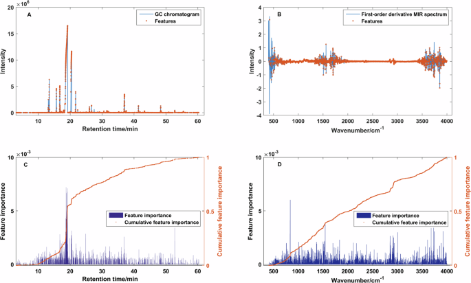
Presentation of important variables using RF method from GC data (A), first-derivative MIR data (B), feature importance and cumulative feature importance plots of GC (C), and first-derivative MIR data (D).

Full size image

Discrimination analysis

The aim of this study was to develop an effective method for discriminating among Chenpi samples harvested from eight regions. The models discussed in materials and methods section were established based on the calibration set, and statistical metrics were estimated using the test set. Five-fold cross-validation was employed for the models, and the hyperparameters are listed in Table 2. The values of these metrics are summarized in Table 3. The discrimination performance of each established model will be discussed in the following sections. At the same time, we supplemented the final model with 1000 permutation tests (Supplementary Table S1).

Discrimination analysis based on single dataset

First, the discrimination of the Chenpi samples was performed using the individual GC data and first-derivative MIR data using AdaBoost, NB, KNN, and ANN. Due to the large number of metrics, here we focus our analysis on the most commonly used metric, accuracy (ACC). Table 3 indicates that the average classification accuracy of the test set obtained from the GC data using AdaBoost, NB, KNN, and ANN was 89.97%, 88.37%, 90.28%, and 89.76%, respectively. The average classification accuracy of the test set obtained from the first-derivative MIR data using AdaBoost, NB, KNN, and ANN was 82.29%, 82.85%, 85.07%, and 80.73%, respectively. These results show that the GC data enable higher discrimination accuracy than the first-derivative MIR data. This may be because more component information can be obtained by GC. To clarify the detailed discrimination accuracy of Chenpi samples from each location, confusion matrices of the actual and predicted classifications are illustrated in Supplementary Figs. S1 and S2.

The discrimination accuracy of these models is not satisfactory, likely due to the presence of excessive redundant information and noise in the full dataset, which degrade the models’ reliability and accuracy. To improve the model performance, the RF method was employed to extract important variables. The important variables extracted from the GC data and first-derivative MIR data are illustrated in Fig. 2A, B, respectively. Discrimination models were then established using these important variables. Table 3 indicates that the discrimination accuracy of the test set obtained from the GC data using the hybrid RF-AdaBoost, RF-NB, RF-KNN, and RF-ANN was 90.42%, 93.75%, 94.44%, and 89.76%, respectively. The discrimination accuracy of the test set obtained from the first-derivative MIR data using the hybrid RF-AdaBoost, RF-NB, RF-KNN, and RF-ANN was 84.37%, 84.45%, 85.07%, and 89.58%, respectively. Except for the RF-ANN model based on the GC data, the prediction accuracy has been improved. These results demonstrate the effectiveness of feature extraction. The confusion matrices of the actual and predicted classifications are illustrated in Supplementary Figs. S3 and S4. The differences between the GC-based and MIR-based results inspired us to improve the discrimination accuracy by using fused data.

Discrimination analysis based on mid-level data fusion

The above analysis indicates that the predictive discrimination accuracy of the hybrid algorithms is better than that of the original algorithms, demonstrating that the RF method effectively extracted important variables. To further improve the discrimination accuracy, the mid-level data fusion strategy was incorporated to enhance the synergy between the integrated information and provide more accurate knowledge about the analyzed samples¹⁷. The fusion of the extracted features is illustrated in Fig. 3A and the average accuracy of the data fusion models is summarized in Table 3. The application of the data fusion strategy results in an average accuracy of 97.29%, 92.86%, and 94.45% using AdaBoost, NB, and KNN. These values are better than those obtained using the non-fused data. This demonstrates the effectiveness of mid-level data fusion, despite the discrimination accuracy of the ANN model (88.20%) being worse than that of RF-ANN. The confusion matrices of the actual and predicted classifications for the test set are illustrated in Fig. 4. In this figure, the vertical axis displays the actual origin classifications of the Chenpi samples, while the horizontal axis shows the predicted origins of Chenpi by the model. The elements on the main diagonal represent the number of correct predictions, with each diagonal element indicating the count of Chenpi samples from a specific origin correctly classified as that origin. This figure clearly demonstrates the prediction accuracy of the algorithm model for each origin.

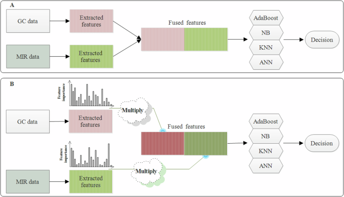
Mid-level data fusion scheme (A) and modified mid-level data fusion (B).

Full size image

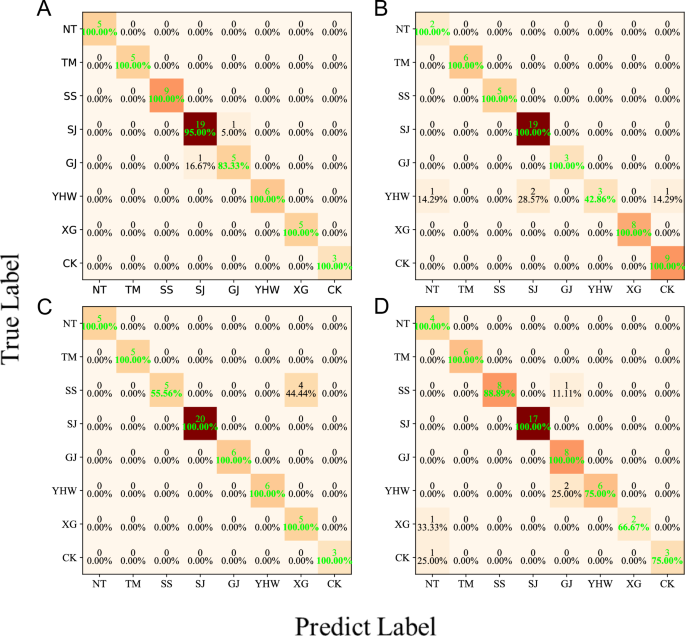
Confusion matrix of the detailed actual and predicted classifications of the test set using AdaBoost (A), NB (B), KNN (C), and ANN (D) on the basis of mid-level data fusion. *The following abbreviations represent place names: NT for Nantan, TM for Tianma, SS for Shuangshui, SJ for Sanjiang, GJ for Gujing, YHW for Yinhuwan, XG for Xiaogang, CK for Chakeng.

Full size image

Discrimination analysis based on modified mid-level data fusion dataset

While mid-level data fusion produces satisfactory results, it does not account for the feature importance of each extracted feature. Since feature importance may affect the discrimination accuracy, the modified mid-level data fusion process illustrated in Fig. 3B was applied. The average accuracy of the modified mid-level data fusion models is summarized in Table 3. The application of the modified mid-level data fusion strategy enhances the discrimination accuracy of the AdaBoost, NB, KNN, and ANN algorithms to 97.27%, 95.51%, 99.37%, and 95.84%, respectively. These values are better than those obtained from the original algorithms, hybrid algorithms, and the mid-level data fusion strategy. The confusion matrices of the actual and predicted classifications for the test set are illustrated in Fig. 5. A detailed comparison of Figs. 4 and 5 indicates that the discrimination results of AdaBoost are not affected by the data fusion method (Fig. 4A and Fig. 5A). As can be seen from Figs. 4B and 5B, although the discrimination accuracy of the NB model using mid-level data fusion is reduced for Sanjiang (SJ) samples, the accuracy is improved for Yinhuwan (YHW) samples, which generally improves the average classification accuracy. Figures 4C and 5C show that the situation is the same for the KNN model. Finally, as can be seen from Figs. 4D and 5D, the discrimination accuracy of the ANN model using modified mid-level data fusion has been greatly improved, with the samples from seven production areas (NT, TM, SS, SJ, GJ, YHW, and CK) classified with 100% accuracy. Moreover, as can be seen from Fig. 5C, D, although the average accuracy of the ANN model is lower than that of the KNN model, both models misclassified only one sample when using the modified mid-level data fusion, demonstrating comparable discrimination performance. The lower average accuracy of the ANN model is due to the misclassified sample belonging to a category with fewer samples, which reduces the overall discrimination accuracy.

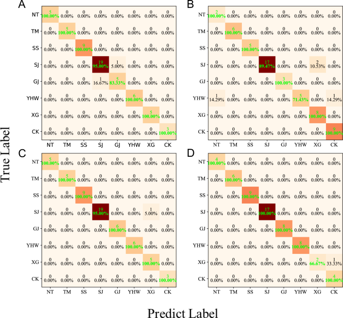
Confusion matrix of the detailed actual and predicted classifications of the test set using AdaBoost (A), NB (B), KNN (C), and ANN (D) on the basis of modified mid-level data fusion. *Abbreviations are the same as in Fig. 4.

Full size image

The results above demonstrate that both the mid-level and modified mid-level data fusion strategies offer a good improvement in discrimination compared to using the individual GC or first-derivative MIR data alone. The KNN and ANN models combined with the modified mid-level data fusion method show superior performance over other models, highlighting the effectiveness of integrating GC and MIR data with advanced machine learning methods for accurately determining the geographical origin of Chenpi.

Although effective discrimination method has been developed, the present study encountered limitations in identifying region-specific components due to challenges in both GC and MIR analyses. In the GC analysis, characteristic variables were dispersed, reducing accuracy in compound identification. Similarly, our current MIR analysis showed no clear correlation between key compounds and Chenpi production areas. In addition to considering the lack of distinct components due to the close geographical proximity of the regions, more effective feature extraction methods are also needed. Literature indicates that deep learning algorithms for functional group prediction from infrared spectra could address these challenges²⁶. To improve the extraction and interpretation of feature information in relation to compounds, we will apply deep learning techniques to automatically identify characteristics information and relationships within spectral data. By employing advanced deep learning methods, we aim to overcome current limitations and accurately identify characteristic compounds associated with different origins, thus enhancing our analysis of regional specificity.

In the future study, we plan to expand the sample size by obtaining Chenpi samples from different provinces to evaluate the robustness of the current approach on a larger dataset. Additionally, we will focus on the development of deep learning methods with advanced feature extraction capabilities, enabling a more detailed analysis of chemical components tied to Chenpi origin to establish a stronger chemical basis for origin discrimination of Chenpi.

Data

The 39 Guangchenpi samples were collected from eight different locations in Xinhui district, namely Nantan (4 samples), Tianma (4 samples), Shuangshui (4 samples), Sanjiang (12 samples), Gujing (4 samples), Yinhuwan (4 samples), Xiaogang (3 samples), and Chakeng (4 samples). Detailed data relating to the samples are presented in Supplementary Table S2. After the purchase of these samples, the experimental analysis was carried out as soon as possible to minimize the impact of external factors on the subsequent results.

The MIR analysis was performed using a Fourier transform infrared spectral analyzer (FTIR, Nicolet iS5, Thermo Fisher Scientific Inc., USA). The samples were pre-treated, milled and then sieved using a 60 sieve. The FTIR spectrum of the Chenpi powder was obtained using the potassium bromide (KBr) pellet method, with KBr purchased from Shanghai Macklin Biochemical Co., Ltd, Shanghai, China. Each sample was weighted to 1 mg, thoroughly mixed with 100 mg of KBr, and pressed into a transparent pellet for analysis. The infrared spectroscopy analysis was performed using OMNIC software, with a scanning range of 400–4000 cm⁻¹, a resolution of 4 cm⁻¹, and 16 times. Each sample was measured in parallel six times, giving a total of 234 data (39 samples ×6 determinations).

The GC analysis was performed on a gas chromatograph-mass spectrometer (GC-MS, 8890-5977B, Agilent Technologies, Inc., USA). The GC separation was conducted using a fused-silica HP-5 MS capillary column with dimensions of 30 m ×0.25 mm i.d. ×0.25 μm. The chromatographic conditions were as follows: the heating program was divided into stages: (I) the initial temperature was set at 35 °C and maintained for 5 min, then raised to 120 °C at a rate of 3 °C min⁻¹, held for 3 min; (II) further heating to 200 °C at 5 °C min⁻¹ and finally ramped to 280 °C at 10 °C min⁻¹. Other parameters included: high-purity helium as the carrier gas at a flow rate of 1.0 mL min⁻¹, injection volume of 1.0 μL, vaporizer temperature set to 280 °C, transmission line temperature at 280 °C, and a split ratio of 1:20. As for the GC analysis, each sample was measured in parallel six times, also giving a total of 234 data.

Variable selection methods

The redundant information in the extracted spectral data can decrease the accuracy of the established model. Variable selection is an effective means of extracting more important information about the target compounds from the full spectral response^27,28. Therefore, selecting a limited number of key variables is recommended to develop more accurate and reliable quantitative and classification models.

The random forest (RF) ensemble algorithm can assess the importance of input variables, with higher contributions variables are more significant, and vice versa²⁹. Therefore, the RF method enables feature selection based on variable importance. In the present study, the RF algorithm was applied to identify important effective variables, thus reducing the complexity and improving the accuracy of the classification models. The RF algorithm was compiled in Python, specifically the Anaconda and sklearn modules. The numpy array object of feature lines was obtained by calling the “feature-e_importance” parameter in sklearn; the sum of the elements in the array is constrained to be 1. Thus, the important variables were extracted from the GC data and first-derivative MIR data.

Classification methods

Machine learning technologies are being applied in a wide range of fields. In the present study, adaptive boosting (AdaBoost), naïve Bayes (NB), K-nearest neighbors (KNN), and an artificial neural network (ANN) were used to establish different models for the classification of samples in accordance with their geographical origin. A brief introduction to each method is now given.

AdaBoost is an iterative algorithm that adjusts the sample weights to form a series of weak classifiers. The core idea is to train a base classifier first, then integrate all the generated classifiers to form a strong classifier³⁰. The weight of each sample is determined according to whether the classification of each sample in the training set is correct and the accuracy of the overall classification³¹. In each training iteration, greater weights are assigned to misclassified samples from the previously weak classifiers; while lower weights are given to correctly classified samples. This adjustment increases the emphasis on misclassified samples in the next iteration, enhancing the model’s focus on challenging cases. New samples are subsequently classified by the ensemble of the trained weak classifiers using majority voting to obtain a final decision³².

NB is one of the most effective and efficient classification algorithms. As indicated by its name, NB is based on Bayes’ theorem, and assumes that all features are independent of each other³³. Using Bayes’ rule, the prior probabilities of each attribute within each class are calculated, allowing classification based on the known probabilities of each class and attribute³⁴.

The KNN algorithm is a nonparametric classifier that operates based on Euclidean distance³⁵. It calculates the distances between unknown objects and each object in the calibration set³⁶, then sorted these distances in increasing order. The core idea of the KNN algorithm is to find the nearest K samples to the unknown samples, and then assign the unknown samples to the class to which most of the K samples belong³⁷.

ANNs are an interconnected assembly of simple processing elements derived through artificial intelligence³⁸. In the present study, a multilayer perceptron (MLP) using backpropagation is applied to establish a neural network model. The MLP is a feed-forward supervised learning network composed of an input layer, a hidden layer, and an output layer³⁹. It adapt its knowledge by adjusting weights on the basis of the classification error of one or more outputs⁴⁰.

These four procedures were implemented using the sklearn program incorporated in the Python software package. Parameter ranges including the default values given in the sklearn Python platform were tested to find the optimum values.

To test the robustness and compare the performance characteristics of the classification models, the original 234 data (39 samples ×6 parallel determinations) were split into a calibration set containing 175 data (75%) and a test set containing the other 59 data (25%). The samples were randomly divided for each model. The calibration set was applied to generate discrimination models and the test set was used to evaluate the prediction performance.

Mid-level and modified mid-level data fusion

Data fusion is an important method in pattern recognition and other fields. Mid-level data fusion often performs better than low-level and high-level data fusion strategies¹⁷. In mid-level data fusion, variable selection is firstly performed to extract relevant information from the original data, after which the selected features are used to form a new matrix⁴¹, largely reducing the influence of irrelevant variables. The mid-level data fusion procedure is illustrated in Fig. 3A.

The present study proposes a novel modified mid-level data fusion strategy. The attention mechanism is inspired by the human vision system, where humans focus on specific regions of an image during recognition⁴². Motivated by this, the attention mechanism assigns varying weights to different regions, focusing more on information that contributes significantly to the current task and assign it a higher weight⁴³. As can be seen from Fig. 2C, D, each extracted feature has a corresponding importance score. To assign higher weights to features with greater importance scores, the attention mechanism is applied. Here, the feature variables extracted from GC data and first-derivative MIR data are weighted by their corresponding feature importance, and a new matrix is then concatenated. The modified mid-level data fusion scheme is illustrated in Fig. 3B. Although other modified mid-level data fusion procedures have been reported, such as the fusion of important features extracted by different methods^44,45 and the assembly of classifiers into the fusion input matrix⁴⁶, our method does not overlap with any existing approaches, making it relatively innovative.

Performance evaluation

The concept of a confusion matrix is used in machine learning to present information about the actual and predicted performance of a classification approach⁴⁷. A confusion matrix has two dimensions, one dimension indexed by the actual class of an object and the other indexed by the predicted class. The data in this matrix provides the basis for evaluating classification performance through various statistical metrics, such as accuracy, precision, sensitivity, and F1 Score, enabling a comprehensive assessment of the model’s effectiveness⁴⁸. The corresponding descriptions were provided as follows:

Accuracy (ACC), represents the proportion of correctly classified samples among the total samples, serves as a general measure of the classifier’s effectiveness.

Sensitivity (SE), or the true positive rate, measures the proportion of actual positives correctly identified by the test. It is critical for ensuring that few cases of the condition are missed. Sensitivity is crucial in medical testing where failing to identify a condition could have severe consequences.

Specificity (SP), or the true negative rate, measures the proportion of actual negatives that are correctly identified. This is particularly important in fields where the cost of a false positive is high.

Precision (Pre), often referred to as the positive predictive value, measures the accuracy of positive predictions. It evaluates the proportion of positive identifications that were actually correct and is especially useful when the costs of false positives are high.

F1 Score (F1) is the harmonic mean of Precision and Sensitivity (Recall), providing a single metric that balances both the concerns of precision and the need for recall. The F1 Score is particularly useful when you need to compare two or more classifiers and when there is an uneven class distribution.

The mathematical formulation⁴⁹ was represented as

where,

True Positive (TP): the model correctly identifies a sample as belonging to the target class.

True Negative (TN): the model correctly identifies a sample as not belonging to the target class.

False Positive (FP): the model incorrectly classifies a sample from a different class as belonging to the target class.

False Negative (FN): the model incorrectly classifies a sample from the target class as not belong to it.

In addition to accuracy, the Area Under the Receiver Operating Characteristic Curve (AUC) is another crucial metric for evaluating the performance of classification models. The ROC curve is a graphical plot that illustrates the diagnostic ability of a binary classifier system as its discrimination threshold is varied. It is created by plotting the true positive rate (TPR), also known as sensitivity, against the false positive rate (FPR), or 1-specificity, for various threshold settings. The AUC represents the degree to which the model is capable of distinguishing between classes. An AUC of 1 indicates a perfect model that correctly classifies all positive and negative instances. Conversely, an AUC of 0.5 suggests no discriminative ability, akin to random guessing. High AUC values, approaching 1, denote a model with high predictive accuracy, which reliably identifies positive and negative cases across the spectrum of threshold levels.

Cohen’s Kappa coefficient is a robust statistical metric used to measure the inter-rater agreement for qualitative (categorical) items, distinguishing it from mere chance agreement. This metric adjusts the accuracy by accounting for the agreement that occurs by chance, making it particularly useful in the analysis of imbalanced datasets. Kappa values range from −1 (total disagreement) to 1 (perfect agreement), with 0 indicating that the agreement is no better than chance. Cohen’s Kappa is calculated using the formula⁵⁰:

where P_o (observed agreement proportion) is represented by the overall accuracy, which is the proportion of instances correctly classified. P_e (expected agreement by chance) is calculated as⁵¹:

where P_row1 and P_row2 are the sums of the rows of the confusion matrix, representing the total actual instances for each class. P_cow1 and P_cow2 are the sums of the columns of the confusion matrix, indicating the total predicted instances for each class. n is the total number of observations.