GLEAM4: global land evaporation and soil moisture dataset at 0.1° resolution from 1980 to near present

Terrestrial evaporation (E) or ‘evapotranspiration’¹ plays a crucial role in the climate system as a nexus between the water, carbon, and energy cycles, reacting to changes in anthropogenic emissions and propagating their influence throughout the global hydrological cycle. It regulates long-term precipitation and temperature projections through its influence on the water vapour, lapse rate and cloud feedbacks, and it influences the occurrence of extreme events, such as droughts, floods and heatwaves^2,3. For water management, E is a net loss of available resources that must be monitored, and for agriculture, crop transpiration determines irrigation needs⁴. Despite this importance, E is highly uncertain at regional and global scales, especially regarding long-term trends and responses to short-term climate anomalies^5,6,7,8. This uncertainty arises because E is (i) rarely measured in the field, (ii) challenging to model accurately (as it involves both plant physiological responses and complex turbulent atmospheric processes), and (iii) invisible to satellite sensors (despite its imprint on surface water and energy balance)⁹. The critical yet uncertain nature of E has spurred innovative attempts to combine in situ, satellite, and reanalysis data to estimate global E. Since over a decade ago, myriad approaches to derive global E datasets have been proposed^10,11,12, often based on the application of prognostic models originally designed for regional scales^13,14,15. Machine learning models trained on eddy-covariance measurements have also been used to represent E globally, leveraging both satellite and in situ data^16,17. However, pure machine learning-based approaches do not explicitly obey physical limits, and their black-box nature complicates interpretability and process understanding¹⁸. An emerging research direction is to combine both physics-based and machine learning models in a synergistic manner, to yield what is frequently referred to as ‘hybrid models’ and which has already met some success in E modelling^19,20,21,22.

The Global Land Evaporation Amsterdam Model (GLEAM¹⁰), one of the first prognostic approaches developed to estimate E globally using satellite data, remains freely available and widely used, with over 10,000 independent users over the past decade²³. GLEAM data are updated to near present at least once a year, and include not just E, but also its different component fluxes (or sources): transpiration (evaporation of water within the leaves), interception loss (from wet surfaces), bare soil evaporation (within soil pores), evaporation from inland water bodies, and evaporation from snow-covered surfaces (typically, yet inaccurately, referred to as ‘sublimation’¹). The dataset also includes other related variables, such as (surface and root-zone) soil moisture, potential evaporation, and evaporative stress. GLEAM data have been used for a wide range of purposes, including the quantification of water resources, driving basin-scale hydrological models, studying global climate trends, and benchmarking climate models²³. Over the years, extensive evaluations of GLEAM against in situ observations^24,25 and alternative gridded datasets^26,27 have evidenced the consistent performance of the dataset in a wide range of applications²³. Recent improvements in GLEAM have concentrated on the use of machine learning to represent evaporative stress²¹, the depiction of groundwater access by vegetation²⁸, and the characterisation of interception loss²⁹. Here, we unify these efforts and present the fourth generation of the GLEAM algorithm and datasets, GLEAM4, which also features an improved spatial resolution (from 0.25 to 0.1°) and extended record length (1980–2023). In the following sections, the approach is explained with specific emphasis on the novel aspects compared to its predecessor, driving data are introduced, and the resulting global datasets are analysed in terms of spatiotemporal consistency and performance.

The rationale behind GLEAM is to focus exclusively on processes that directly impact E while maintaining a parsimonious approach. The aim is to extract the most relevant information about E from existing Earth observations, incorporating new processes only if they are both crucial and can be effectively constrained by observations. Following this rationale, GLEAM calculates E (and its components) through four sequential steps (or ‘modules’) targeting the computation of (i) interception, (ii) potential evaporation, (iii) soil water content, and (iv) evaporative stress¹⁰. Figure 1 provides a schematic of GLEAM4 together with the input and output variables of each module. First, rainfall interception loss over vegetated surfaces (E_i) and potential evaporation (E_p) are computed. E_p is then converted into actual evaporation (E) using a multiplicative evaporative stress factor (S) that is based on root-zone soil moisture (SM_rz), among other variables²¹. This is done independently for the fraction of bare soil, and the fractions of tall and short vegetation within each pixel, yielding estimates of (actual) bare soil evaporation (E_b) and transpiration (E_t), respectively. To consider understorey bare soil evaporation, GLEAM4 computes the transmission of incoming radiation through the canopy using the Beer-Lambert law based on leaf area index (LAI)³⁰. Finally, E is considered to equate E_p in regions covered with snow and ice (E_s), and open water (E_w), using specific parametrisations for these surfaces¹⁰.

Schematic of GLEAM4. Variable names and data sources are listed in Table 1, and their colour denotes the module in which they are employed.

Full size image

Since the publication of GLEAM version 3 (v3)³¹, several research efforts have concentrated on improving multiple aspects of the modelling framework. These improvements concern each of the four modules in GLEAM, as illustrated in Fig. 1, and have been documented in individual publications over the past few years^21,28,29. Moreover, (i) datasets were extended to near-present, and (ii) spatial resolution was increased from 0.25° to 0.1° thanks to the updates in forcing data. The following provides a general summary of the methodology behind GLEAM4, concentrating on the improvements upon GLEAM v3 and how these affect the estimates of E, its component fluxes, and other related hydroclimatic variables.

Rainfall interception

E_i is computed on rainy days, contributing to E while influencing effective precipitation and soil water content. It remains one of the most uncertain fluxes in the global water cycle, mainly due to the limited availability of in situ campaign data for parameterising (or training) universal models³². In GLEAM4, the previous approach based on Gash’s analytical model³³ is replaced by the approach in ref. ²⁹, which performed a synthesis of interception data from past field experiments conducted worldwide, including campaigns in 166 forest sites and 17 agricultural plots. Based on this meta-analysis, a global van Dijk–Bruijnzeel interception model³⁴ was constrained using satellite-observed vegetation dynamics — i.e., fraction of absorbed photosynthetically active radiation (f PAR) and LAI — potential evaporation, and precipitation data²⁹. This E_i formulation accounts for sub-grid heterogeneity, computing the flux for tall and short vegetation fractions separately, thus improving upon previous GLEAM versions that only included interception for tall vegetation. This improved performance has been demonstrated in validation experiments against field data²⁹ as well as product inter-comparisons³⁵.

Potential evaporation

Unlike previous GLEAM versions, which were based on Priestley and Taylor’s equation¹⁴, GLEAM4 uses Penman’s equation¹³ to explicitly reflect the influence of wind speed (u, m s⁻¹), vegetation height (h, m), and vapour pressure deficit (VPD, Pa) on E_p. The original motivation for using Priestley and Taylor was its minimum input requirements (i.e., net radiation and air temperature), making it well-suited for satellite data applications.¹⁰. However, recent advances in satellite remote sensing and climate reanalysis have yielded observational datasets of h³⁶, u³⁷, and VPD³⁸, making Penman’s approach increasingly suited for purpose. As such, E_p (mm s⁻¹) in GLEAM4 is calculated for each land cover fraction within each pixel as:

where ∆ is the slope of saturation vapour pressure curve (Pa °C⁻¹), R_n is the surface net radiation (W m⁻²), G the ground heat flux (W m⁻²), ρ_a is the air density (kg m⁻³), c_p is the specific heat at constant pressure (J kg⁻¹ °C⁻¹), g_a is the bulk aerodynamic conductance (m s⁻¹), λ is the latent heat of vaporisation of water (J kg⁻¹), and γ is the psychrometric constant (Pa °C⁻¹). ∆, ρ_a, λ and γ are computed as a function of air temperature¹⁰, R_n is partitioned per land cover fraction³¹, and the G/R_n ratio is considered an inverse function of LAI³⁹. g_a is approximated using Thom’s equation⁴⁰, assuming a neutral atmosphere and accounting for the excess resistance of the transfer of vapour compared to momentum⁴¹:

where k is von Kármán’s constant (0.41), z is the height of the u observations (m), d is the zero-plane displacement height (m), and z_0m is the roughness length for momentum (m); d and z_0m are assumed to be 2/3 and 1/10 of h respectively for the non-vegetated fractions⁴², with an additional dependence on LAI for the vegetated fractions⁴¹. The roughness length for vapour (z_0v), which is assumed to be the same for heat (z_0h), is calculated from z_0m via the so-called kB⁻¹ approach, where kB⁻¹ = ln(z_0m/z_0h) is a vegetation specific value taking values of 5 and 8 for short and tall vegetation, respectively⁴³.

Soil water

Soil water content across the root depth is required for later computation of evaporative stress (see below). GLEAM uses a multi-layer running water balance driven by precipitation data (and E), which considers a constant root depth per land cover fraction³¹. Microwave soil moisture (SM_s) and/or backscatter observations are assimilated^44,45 in the top soil layer. Plants are assumed to be able to extract water from where it is more easily accessible within the soil profile; thus the wettest soil layer is selected for computing evaporative stress. In nature, groundwater can also be an important source for E, especially during dry conditions and in ecosystems where vegetation has deep roots⁴⁶. Previous versions of GLEAM did not explicitly account for plant access to groundwater. The approach adopted by GLEAM4 uses a linear reservoir model to represent groundwater, and introduces a partitioning of transpiration to estimate groundwater-sourced E²⁸. Validations against field observations of E, soil moisture, discharge and groundwater levels demonstrated a realistic representation of E under water-limited conditions²⁸, enabling the future assimilation of satellite gravimetry data into the model⁴⁷. GLEAM4 assimilates surface soil moisture data from the European Space Agency (ESA) Climate Change Initiative (CCI)⁴⁸ (see Table 1). The data assimilation is based on a Newtonian Nudging scheme where soil moisture is first decomposed into anomalies, and then uncertainties in the latter are computed based on triple collocation³¹.

Evaporative stress

As mentioned above, to constrain E below E_p, GLEAM uses a multiplicative stress factor (S) that ranges from 0 (maximum stress) to 1 (no stress). S is expected to capture all factors that restrain the supply of water to the atmosphere below the atmospheric demand (i.e., E_p). In GLEAM4, the original semi-empirical computation of S based on soil moisture (see above) and vegetation optical depth (VOD)^10,31, is replaced by the deep neural network approach presented in ref. ²¹. The latter acknowledges that the ratio between actual and potential transpiration can be controlled by numerous environmental variables that interact non-linearly, including not just soil moisture and VOD, but also VPD, incoming solar radiation (SW_i), air temperature (T_a), CO₂ concentration, u, and LAI — see Fig. 1. Global eddy-covariance and sapflow data are used to learn universal transpiration stress functions, separately for tall and short vegetation. The neural network formulations of S are embedded within GLEAM4, enabling bidirectional coupling with the process-based model and influencing both E and the soil moisture used to compute S in the next time step. Comparisons against in situ data and satellite-based proxies demonstrated that the hybrid (AI–process-based) approach has an enhanced ability to estimate S and E for most ecosystems compared to previous GLEAM versions²¹.

Input data

Table 1 lists all the input variables and datasets used in the generation of GLEAM4 datasets. Input data have been resampled to a common 0.1° resolution by means of bilinear interpolation, when needed.

Data archive

The GLEAM4 dataset currently amounts to approximately 1.1TB. Data are freely available in a public SFTP server under a CC BY licence, and can be accessed through https://www.gleam.eu/#downloads. For a detailed description of the dataset, we refer readers to the technical notes at https://doi.org/10.5281/zenodo.14056079. The E dataset from the exact sub-version used in this manuscript (v4.2a) can also be found in this repository. Dataset specifications are also found on the GLEAM website and through its Digital Object Identifier (DOI)⁴⁹. The period covered by GLEAM4 is currently 1980–2023 at daily temporal resolution and 0.1° spatial resolution. GLEAM datasets are updated annually (in March–April) and extended until the end of the previous year, as input data become available.

Like in previous versions of GLEAM³¹, two distinct data archives are available that differ on their temporal coverage and reliability on observational data. The archive ‘a’ relies mostly on the reanalysis from Multi-Source Weather (MSWX³⁷) and precipitation from Multi-Source Weighted-Ensemble Precipitation (MSWEP⁵⁰) as forcing data. It covers the entire period 1980–2023, and it is intended for climatological studies requiring longer record lengths. The archive ‘b’ has a more observational nature and a lower reliance on reanalysis due to its use of radiation fluxes from the Clouds and the Earth’s Radiant Energy System (CERES⁵¹), precipitation from Integrated Multi-satellite Retrievals for the Global Precipitation Mission (IMERG⁵²), and temperature and VPD from the Atmospheric Infrared Sounder (AIRS³⁸). Its record length is however shorter, currently spanning the period 2003–2023. Table 1 lists the specific datasets used to generate both data archives.

The following 12 variables are available for each of the two data archives (‘a’ and ‘b’):

Actual evaporation (E, mm day⁻¹)

Transpiration (E_t, mm day⁻¹)

Bare soil evaporation (E_b, mm day⁻¹)

Interception loss (E_i, mm day⁻¹)

Open-water evaporation (E_w, mm day⁻¹)

Condensation (E_c, mm day⁻¹)

Evaporation over snow and ice (E_s, mm day⁻¹)

Potential evaporation (E_p, mm day⁻¹)

Evaporative stress (S, unitless)

Surface soil moisture (SM_s, m³ m⁻³)

Root-zone soil moisture (SM_rz, m³ m⁻³)

Surface sensible heat flux (H, W m⁻²)

Data structure

Data are organized into netCDF files, with one file per variable per year. Each daily file contains a 3D array with dimensions n × 1800 × 3600, where n is the number of days in the respective year, 1800 is the number of grid cells in the latitudinal dimension, and 3600 is the number of grid cells in the longitudinal dimension. The first cell in each file corresponds to January 1st of that year, centred at latitude 89.95^° and longitude –179.95^°. In addition to daily data, netCDF files containing monthly (dimensions 12 × 1800 × 3600) and annual (dimensions 1 × 1800 × 3600) means are also available.

These datasets are stored on the public server in the following directory structure: <ARCHIVE>/<TEMPORAL_RESOLUTION>/, where <ARCHIVE> refers to either GLEAM4.2a (v4.2a) or GLEAM4.2b (v4.2b), <TEMPORAL_RESOLUTION> indicates the temporal aggregation level (‘daily’, ‘monthly’, or ‘yearly’), and ‘v4.2’ indicates the subversion of the GLEAM4 dataset. Daily datasets are organized by year, while monthly and yearly datasets are organized by variable.

Daily files follow this naming convention: <VARIABLE>_<YEAR>_GLEAM_<ARCHIVE>.nc, where <VARIABLE> corresponds to the variable names listed in the previous section: ‘E’, ‘Et’, ‘Eb’, ‘Ei’, ‘Ew’, ‘Ec’, ‘Es’, ‘Ep’, ‘S’, ‘SMrz’, ‘SMs’, ‘H’, and <YEAR> is the four-digit year. For example, a file containing daily evaporation data for 2023 in the ‘a’ dataset would be named:

v4.2a/daily/2023/E_2023_GLEAM_v4.2a.nc.

Monthly and yearly files follow this naming convention: <VARIABLE>_<YEAR>_GLEAM_<ARCHIVE>_<TEMPORAL_RESOLUTION>.nc, where <TEMPORAL_RESOLUTION> is abbreviated as ‘MO’ for monthly or ‘YR’ for yearly. For monthly and yearly files, flux units are mm month⁻¹ and mm year⁻¹, respectively, instead of mm day⁻¹. For example, a file containing monthly root-zone soil moisture data for 2010 from the ‘b’ archive would be named:

v4.2b/monthly/SMrz/SMrz_2010_GLEAM_v4.2b_MO.nc.

Global patterns

Figure 2 explores mean global E patterns (1980–2023), along with the absolute and relative contributions from different component fluxes. Unless otherwise noted, GLEAM4 corresponds to the v4.2a data, the latest subversion at the time of writing this manuscript. As expected, E_t dominates the flux globally, especially in densely vegetated humid tropics due to year-round soil water availability and high incoming radiation. The global proportion of E originating from E_t is 62%, falling within the envelope of current global estimates⁵³, but below the 74% from GLEAM v3³¹, which was on the high end of the spectrum of globally available products. The reduction of E_t from GLEAM v3 to GLEAM4, results from the consideration of short vegetation interception loss and understorey bare soil evaporation in GLEAM4, among other methodological improvements (see Methods). E_i constitutes 14% of the global flux, being larger in forested regions, as expected, while E_b amounts to 17% of global E and is larger in sparsely vegetated regions. Negative estimates in GLEAM4 indicate condensation and are illustrated together with other minor components (i.e., snow and open-water evaporation) in Fig. 2. The mean E in GLEAM4 is 68.5 × 10³ km³ yr⁻¹, which agrees with state-of-the-art water cycle appraisals based on extensive literature meta-analysis⁸ (69.2 ± 7 × 10³ km³ yr⁻¹) and with other global observational datasets (see below).

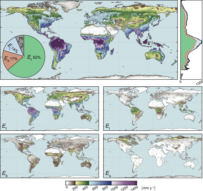
Mean evaporation and its components. Long-term (1980–2023) mean terrestrial evaporation (E) (top). The global decomposition of its component fluxes is shown in the pie diagram and the latitudinal profile on the right. Long-term means for each of the components (bottom): transpiration (E_t), interception loss (E_i), soil evaporation (E_b), and other sources (E_o), including snow sublimation (E_s), open water evaporation (E_w), and condensation (E_c). All fluxes are in mm yr⁻¹.

Full size image

The seasonal dynamics of some of the key variables from GLEAM4 are portrayed in Fig. 3. The sub-panels showcase global multi-year (1980–2023) mean E, E_p, S, SM_rz, and H during boreal summer (June, July, August), and boreal winter (December, January, February). The seasonal pattern of E_p aligns primarily with the cycle of net radiation, while E is additionally determined by the seasonality of SM_rz, and thus precipitation. Subtropical regions with sufficient JJA precipitation (e.g., India, Northern Australia, parts of Southern Africa, or the east coast of the United States) exhibit the most significant variations in E, with summer E often being an order of magnitude larger than winter levels. In more arid regions, such as central Australia or the Arabian Peninsula, where rainfall occurrences are rare, the seasonal volumes of E remain persistently low throughout the year and unaffected by the E_p cycle. In these areas, the dissipation of available energy primarily occurs through H due to limited SM_rz and E. Likewise, E is persistently low in permanent snow regions, despite higher values during the high-radiation season. Overall, these seasonal patterns agree with relevant literature^{26,54,55,56,57}.

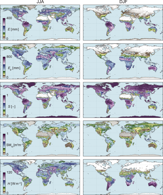
Seasonal patterns. Long-term (1980–2023) means for June, July, and August (JJA, left) and December, January, and February (DJF, right) for terrestrial evaporation (E, mm), potential evaporation (E_p, mm), evaporative stress (S = E/E_p, –), root-zone soil moisture (SM_rz, m³ m⁻³), and surface sensible heat flux (H, W m⁻²).

Full size image

Understanding the dependency of E on different driving factors can provide crucial insights into the seasonal behaviour of E in specific regions, and potentially into the main controls on long-term E trends⁵⁸. Figure 4 provides an overview of these driving factors, leveraging from the partitioning of potential evaporation into an aerodynamic and a radiative term in Penman’s combination equation (see Eq. 1), and taking advantage of the separate calculation of evaporative stress in GLEAM4 (see Methods). Red tones in semiarid regions indicate the dominance of evaporative deficit (E – E_p); in these regions, precipitation supply is insufficient to satisfy the high atmospheric demand for water. On the other hand, in temperate and boreal forests, precipitation supply is sufficient to meet the atmospheric demand; in particular, the aerodynamic component of E_p (which depends on wind, turbulence, ecosystem height and VPD) shows a higher relevance, as shown by the green tones. In the tropics, E_p is primarily satisfied by the radiative component of E (blue tones), which is high due to the high incoming radiation and low albedo of rainforests. Globally, the atmosphere demand for water, or E_p, adds up to 151 × 10³ km³ yr⁻¹, of which ∼55% is unsatisfied (evaporative deficit), and the remaining is satisfied by E through radiative (∼31%) and aerodynamic (∼14%) processes.

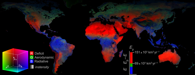
Evaporation control factors. Relative importance of radiative energy (left-hand term in Eq. 1), aerodynamics (right-hand term in Eq. 1), and evaporative deficit (E_p − E), based on long-term (1980–2023) mean fluxes. The bar diagram indicates the global (area-weighted) mean of each term.

Full size image

Validation and inter-comparison

Figure 5 shows a comparison of GLEAM4 E against frequently used global E datasets, including its immediate predecessor GLEAM v3.8a³¹, the ERA5-Land reanalysis⁵⁹, and FLUXCOM (RS-METEO)⁵⁶. Long-term means for all datasets portray similar geographical patterns, with GLEAM4 showing greater agreement with ERA5-Land and FLUXCOM in the tropics compared to GLEAM v3.8a, largely due to a decrease in transpiration estimates over rainforests (as seen in the comparison between Fig. 2 and the results in ref. ³¹). Regional differences indicate relatively high values of GLEAM4 compared to other products in temperate and boreal forests in the Northern Hemisphere, where the consideration of the aerodynamic term of Penman’s Eq. (1) in the new version results in higher E_p and subsequently higher E than in GLEAM v3.8a. Relatively low estimates by GLEAM4 are concentrated in semiarid ecosystems — such as western United States, southern Africa or the Mediterranean region — especially when compared to FLUXCOM and ERA5-Land. This reflects the fact that the evaporative stress in GLEAM4 under water-limited conditions is greater than for GLEAM v3.8a, regardless of the generally larger atmospheric demand for water in the former (as seen in the comparison between E_p in Fig. 3 and the results in ref. ⁵⁵).

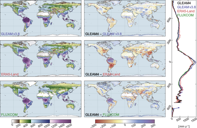
Global inter-comparison of E estimates from different datasets. The left column shows long-term means for GLEAM v3.8a³¹, ERA5-Land⁵⁹, and FLUXCOM⁵⁶ for their common period (1980–2020). The difference between them and GLEAM4 is shown on the right, along with the mean latitudinal profile for all four datasets.

Full size image

The global mean estimates of E from the four datasets are comparable, ranging from highest to lowest: 72.8, 71.8, 68.5 and 67.7 × 10³ km³ yr⁻¹, for ERA5-Land, GLEAM v3.8a, GLEAM4 and FLUXCOM, respectively. As indicated above, these estimates fall within the range of a recent meta-analysis⁸ that reported 69.2 ± 7 × 10³ km³ yr⁻¹.

At regional scales, the patterns of GLEAM4 appear realistic and highlight the value of transitioning to higher spatial resolutions to better capture the influence of complex topography and land use changes. Figure 6 compares the estimates from GLEAM4 to those from the other three datasets during two of the most significant summer droughts in the historical record: the 1988 North American drought⁶⁰ and the 2003 European drought⁶¹, both of which were compounded by severe heatwaves. During drought and heatwave events, E tends to exhibit positive anomalies in the early stages, as long as soil moisture remains sufficiently available, due to the high atmospheric demand for water (E_p). However, as these events progress and soil moisture depletion leads to increased evaporative stress (S), anomalies typically become negative, triggering feedback mechanisms that can further intensify the events². Whether anomalies are overall positive or negative when integrated across the event largely depends on initial soil moisture conditions and the duration and severity of the event⁷. The four datasets evaluated in Fig. 6 appear to capture this complex interplay between water supply and demand, showing good agreement in the regional distribution of positive and negative anomalies. The coarser resolution of FLUXCOM is evident, and so are its reported difficulties in capturing the magnitude of anomalies. However, the recently released next generation of FLUXCOM datasets employs higher resolution and may offer improved capabilities for capturing anomalies during such events¹⁷.

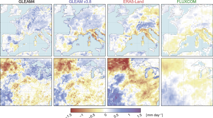
Regional inter-comparison during summer droughts. Top figures refer to the E anomalies during the 2003 summer (JJA) European drought. Bottom figures show E anomalies during the 1988 summer (JJA) North American drought. From the left to right: GLEAM4, GLEAM v3.8a³¹, ERA5-Land⁵⁹, and FLUXCOM⁵⁶ at their original resolution (i.e., 0.1°, 0.25°, 0.1°, 0.5°, respectively).

Full size image

To evaluate the skill of GLEAM4 in capturing temporal dynamics at the ecosystem scale, E estimates are validated against in situ eddy-covariance data from a wide range of global networks, including FLUXNET La Thuile, FLUXNET2015, FLUXNET-CH4, AmeriFlux, ICOS, and EFDC²¹. For duplicate stations across sources, the longest record was retained. Subsequently, sites with fewer than 250 days were excluded. This yielded a final sample of 473 sites and 2511 years of data. Figure 7 compares the overall performance of the four datasets GLEAM4 and the other three datasets (i.e., GLEAM v3.8a, ERA5-Land, and FLUXCOM) in simulating E. Results are illustrated through Taylor density diagrams and violin plots of Kling-Gupta Efficiency (KGE), both displaying the distribution of the validation metrics that are calculated per site. The normalised standard deviation (std) in the Taylor diagrams indicates a mild tendency of all datasets (except for ERA5-Land) to underestimate the variability of E times series, which could relate to their large pixel coverage compared to the more reduced tower footprint. Median root-mean-square error (RMSE) and Pearson’s correlations (R) are similar for all datasets, but slightly better for FLUXCOM (0.89 mm d⁻¹, 0.77) than for GLEAM4 (0.95 mm d⁻¹, 0.73) and ERA5-Land (1.0 mm d⁻¹, 0.77). Meanwhile, KGE values — integrating correlation, variability and bias — show higher median values (and thus better performance) for GLEAM4 than for ERA5-Land (0.49 vs.0.45), and a slight improvement upon GLEAM v3.8a (0.48).

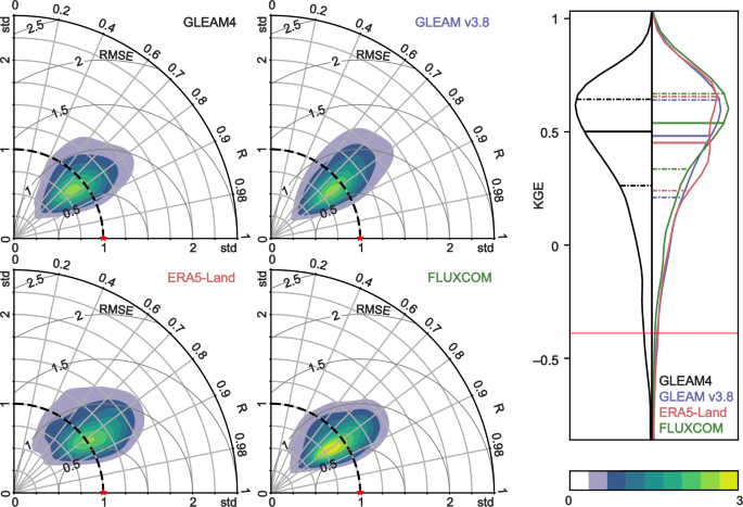
Validation using in situ eddy-covariance measurements. Density Taylor diagrams for the validation of GLEAM4, GLEAM v3.8a³¹, ERA5-Land⁵⁹, and FLUXCOM⁵⁶ against in situ data (left). Normalized standard deviation (std), Pearson’s correlation (R) and centred pattern root mean square error (RMSE) are shown. The ideal performance is marked with a red star. Gaussian Kernel density functions are used to estimate the probability density of data points in the polar space (defined by R and std), thus contour levels indicate unitless thresholds of density values. Violin plots of Kling–Gupta Efficiency for the four datasets (right). Median and interquartile ranges are marked with continuous and discontinuous lines, respectively. Validation based on data from 473 sites.

Full size image

Figure 8 zooms into example time series at four specific sites. The sites correspond to the Tharandt spruce forest in Eastern Germany (DE-Tha), a rainfed maize-soybean rotation site in Nebraska (US-Ne3), the Australian open woodland savanna site in Howard Springs (AU-How), and the French evergreen Mediterranean forest in Puechabon (FR-Pue). These sites were selected based on their long records (>10 years) which allow the reliable computation of seasonal climatologies. Years were selected based on extreme conditions: droughts for FR-Pue⁶² and US-Ne3⁶³, heatwaves for DE-Tha⁶⁴, and pluvial events for AU-How⁶⁵. The left time series indicate anomalies in E, computed by subtracting the seasonal climatology of the corresponding dataset, using a multiyear mean for each calendar day and a 31-day moving average to compute that climatology⁶⁶. Time series of anomalies show significant fluctuations across seasons and climatic events, and often differences among the different datasets, but also remarkable similarities among them and when compared to the in situ data. This pattern is observed at all four stations. While simulating correctly the seasonal cycles may in principle seem like a trivial task compared to simulating temporal anomalies accurately, the smaller panels on the right indicate that the different products still struggle to simulate the seasonality of E. This could relate to differences in land cover from the tower footprint to the coarser-resolution pixels, and it is also influenced by biases in the input data used by each of the models. Nonetheless, all datasets capture the timing of the seasonal cycle, but overestimate its amplitude in DE-Tha and FR-Pue, while they show a larger divergence in general and a tendency to underestimate in both US-Ne3 and AU-How. Overall, GLEAM4 aligns well with observed seasonal cycles, and despite the heterogeneous performance across sites, it reproduces E anomalies across diverse climates and ecosystems successfully, even during extreme events like the ones depicted in Fig. 8.

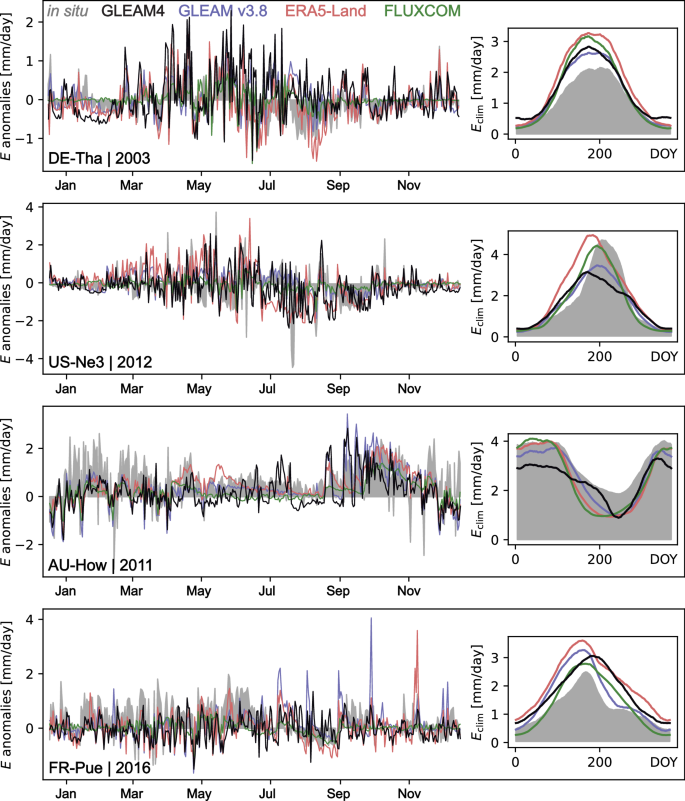
Example time series. Time series for GLEAM4, GLEAM v3.8a³¹, ERA5-Land⁵⁹, and FLUXCOM⁵⁶ against in situ data from four sample sites during a selection of extreme years. Left plots indicate anomalies in E while the right plots show the seasonal climatology for each day of the year (DOY).

Full size image