Health assessment and health trend prediction of wind turbine bearing based on BO-BiLSTM model

    Grid-connected wind turbines need to operate in harsh environments for a long time. Due to long-term uninterrupted operation and the impact of extreme weather, rainfall, snow, and other factors, over time, the health and reliability of each component of the wind turbine will deteriorate. Performance will inevitably degrade, eventually leading to failure¹. Multiple studies have shown that the main sources of wind turbine failures include key components such as high-speed shafts, low-speed shafts, gearboxes in the wind turbine transmission system, and generators and pitch control systems in the electrical system. The maintenance costs of these failures will directly affect the economic benefits of wind farms².

Equipment health status assessment involves modeling the performance degradation state using condition monitoring data and constructing a one-dimensional Health Index (HI) curve to characterize the equipment performance degradation process³. As the operating time of wind turbines increases, the health status of key components in the transmission system, such as bearings, gradually degrades. Health assessment of bearings refers to the quantitative evaluation of a series of different degradation states of bearings from an intact state to an initial fault state and until complete failure. The constructed HI curve should be able to reflect the degradation process of the equipment in a timely and accurate manner. In recent years, domestic and international scholars have carried out a series of studies on equipment health status assessment and have achieved fruitful results. Literature⁴ extracted time-domain features from the vibration signals of rolling bearings and used a monotonicity index to evaluate the degradation process of each time-domain feature. Literature⁵ eliminates a method based on two-stage updated digital twins and a dual-correlated dynamic graph convolutional network (DC-DGCN) for predicting the remaining useful life of bearings. Literature⁶ used kurtosis to describe the degradation process of the high-speed shaft bearings in wind turbines and applied this index to the remaining life prediction of the high-speed shaft bearings. Literature² used Principal Component Analysis (PCA) for data fusion and took the first principal component with the largest variance to construct the system health index. The degradation features selected in the above literature are too singular, and the constructed HI cannot effectively reflect the degradation process and health status of wind turbine bearings. Literature⁷ constructs a comprehensive evaluation function to select rational degradation features and employs the filtered degradation features to predict the remaining useful life of the equipment. For this reason, it is crucial to construct a comprehensive evaluation function to select excellent time-domain, frequency-domain, and time-frequency domain degradation features, and use the Self-Organizing Map (SOM) network to fuse the selected degradation features, so as to construct the HI curve to characterize the health status of the high-speed shaft bearings in wind turbines.

Based on the established bearing HI, this paper studies the health degradation trend of bearings. The selection of prediction algorithms is another key issue. In the field of prediction, the most widely used intelligent algorithms are mainly machine learning methods and neural network methods, with representative ones including Support Vector Regression (SVR) and BP neural network algorithm, etc. SVR is mainly suitable for prediction problems with a small number of training samples. The SVR algorithm predicts the output corresponding to new input data by fitting regression⁸. However, as the training sample set continues to grow, it will lead to a linear increase in the number of support vectors, which in turn leads to overfitting problems and an increase in computational resources. Compared with SVR, neural networks, as mathematical models that simulate the structure and function of biological neural networks, are more proficient in handling large sample data and possess strong nonlinear fitting capabilities. Neural networks achieve this by increasing the number of hidden layer neurons and selecting appropriate activation functions, which endow them with relatively strong nonlinear fitting abilities. There is considerable flexibility in the selection and adjustment of their structures. However, in practical applications, the adjustment of model parameters is often difficult to determine, and there are drawbacks such as being prone to falling into local minima, which can greatly affect their predictive capabilities. The above-mentioned prediction algorithms do not consider the temporal correlation between data points and assume that there is no correlation between time series, that they are independent of each other. Recurrent Neural Networks (RNN) take into account the feedback information from the previous moment while processing the current input information, hence RNN is more proficient in time series prediction. However, RNN is only suitable for short-term time series prediction because when the number of layers in the loop is large, it will make the RNN training time longer, and it is accompanied by the problem of gradient explosion and gradient disappearance. The Long Short-Term Memory (LSTM) network⁹ is a recurrent neural network improved by Hochreiter and Schmidhuber based on the RNN neural network, which effectively improves the poor long-term prediction performance of RNN. The LSTM network uses past information to infer subsequent information. In time series prediction, the Bidirectional Long Short-Term Memory (Bi-LSTM) network takes into account the patterns of information before and after the prediction time, which can improve prediction accuracy.The Bi-LSTM network is an improved version of the LSTM network, mainly used for processing sequential data, especially in Natural Language Processing (NLP) tasks. Bi-LSTM captures information by processing the input sequence in two directions, thereby utilizing the context information from both the past and the future.

Fan et al.¹⁰ constructed a novel multi-scale time series prediction model, BiLSTM-MLAM, which utilizes Bi-LSTM to capture the information before and after in time series data and enhances feature extraction through a local attention mechanism. Experimental results demonstrate that the model’s predictive performance on multiple datasets is superior to other baseline methods; Li et al.¹¹, when predicting building energy (which is affected by seasons), encountered issues such as low efficiency in hyperparameter optimization and inaccurate predictions. They proposed a method based on Bayesian Optimization (BO), Spatio-Temporal Attention (STA), and LSTM. They compared seven improved LSTM models (BO-LSTM, SA-LSTM, TA-LSTM, STA-LSTM, BO-SA-LSTM, BO-TA-LSTM, and BO-STA-LSTM) with the standard LSTM and analyzed the impact of seasonal variations on BO-STA-LSTM using different sample types and time-domain analyses. The results verified that the model’s performance is better than CNN and TCN, exhibiting excellent predictive accuracy; Lu et al.¹² proposed a submarine cable fault detection method, namely a Bi-LSTM model based on Variational Mode Decomposition (VMD) and self-attention mechanism. According to comparative experiments and ablation studies, the proposed model was proven to be superior to other benchmark models and demonstrated robustness and stability under different signal-to-noise ratio conditions; Wu et al.¹³ used FFT transformation and input the results into an improved Gated Recurrent Unit (GRU) network, incorporating an improved attention mechanism to predict the Remaining Useful Life (RUL) of bearings; Zhang et al.¹⁴ extracted key information from the multi-sensor data of turbofan aero engines using a Bidirectional Gated Recurrent Unit (Bi-GRU) network and input it into a Transformer model for life prediction; He et al.¹⁵ proposed a fine time-shift multi-scale fractional-order fuzzy diagnostic technique, which can accurately diagnose the fault types of train bearings in noisy environments. The above literature indicates that Bi-LSTM networks have significant advantages over traditional RNNs and LSTMs in terms of temporal sequence processing.

Bayesian optimization constructs a surrogate model (such as a Gaussian process, a tree-structured Pareto surrogate model, etc.) to approximate the objective function (i.e., the performance metric of the model, such as the loss on the validation set), and optimizes this surrogate model to guide the search direction of hyperparameters. Compared to traditional grid search or random search, Bayesian optimization can more efficiently find the global optimum. Currently, Bayesian optimization of Bi-LSTM models has been applied in the fields of time series prediction¹⁶ and fault prediction¹⁷. Based on the research of the aforementioned scholars, this paper proposes a hyperparameter optimization algorithm for the Bi-LSTM model based on Bayesian optimization, in order to further improve the prediction accuracy of the Bi-LSTM model and its generalization ability. It is applied to the health degradation trend prediction of bearings, and a comparative analysis of the prediction results with several other algorithms is conducted.

In summary, HI curve and the wind turbine bearing performance evaluation process based on the BO-BiLSTM prediction model mentioned in the first half of this paper are shown in Fig. 1. It is mainly divided into three parts: feature extraction, HI curve construction, and BO-BiLSTM prediction model construction.

High-speed shaft bearing health indicator and trend prediction algorithm construction flow chart.

Full size image

Degenerate feature extraction

    Since the wind turbine is in a harsh operating environment, and the transmission system has multiple components and a complex structure, the vibration signals of each component overlap and interfere with each other. A single feature cannot fully reflect the operation of the wind turbine bearing.

The combination of complementary ensemble empirical mode decomposition (CEEMD) and entropy can fully reflect the operating status of the equipment, so this article selects wind turbine bearing vibration signal CEEMD entropy – time-frequency domain features, as part of the degradation features. This method adds the same number of auxiliary white noises with opposite amplitudes to the signal to be decomposed, which not only solves the previous mode aliasing problem but also reduces the reconstruction error to almost zero.

For wind turbine bearing data, 36 features including time domain, frequency domain, and time-frequency domain of each set of sampling data are extracted^18,19 to reflect the characteristics of high-speed shaft bearings as comprehensively as possible Running status.

Time domain features

    Time domain features are statistical quantities calculated directly from the time series of vibration signals. Let (P) be the vibration signal sequence with (n=1,2,ldots ,N), where (N) is the number of samples. The formulas for calculating time domain features are shown in Table 1.

Frequency domain features

    Frequency domain features are obtained from the signal (x(n)) after Fast Fourier Transform (FFT), resulting in the spectrum (y(k)) where (k=1,2,ldots ,K), (K) is the number of spectral lines, and (f_k) is the frequency value of the (k)-th spectral line. The formulas for calculating frequency domain features are shown in Table 2.

Time-frequency domain features

    Extraction of degradation features is crucial for constructing health indicators and directly affects the accuracy of health assessment. Due to the complex structure of wind turbine drive systems, the vibration signals of various components are superimposed and coupled, exhibiting severe nonlinearity and non-stationarity. The complementary ensemble empirical mode decomposition (CEEMD) combined with entropy can fully reflect the operating state of the equipment. Therefore, this paper extracts the CEEMD entropy of vibration signals as part of the degradation features. This method adds auxiliary white noise of the same magnitude but opposite in sign to the signal to be decomposed, which not only solves the previous mode mixing problem but also reduces the reconstruction error to almost zero²⁰.

The specific steps of CEEMD decomposition are as follows:

1. 1.

   Add white noise of the same magnitude but opposite in sign to the signal (x(t)) to obtain (y_1^+(t)) and (y_1^-(t)):

   $$begin{aligned} y_1^+(t) = x(t) + z_1^-(t) end{aligned}$$

   (1)
   $$begin{aligned} y_1^-(t) = x(t) + z_1^+(t) end{aligned}$$

   (2)
2. 2.

   Perform EMD decomposition on (y_1^+(t)) and (y_1^-(t)) respectively to obtain the corresponding intrinsic mode functions (IMF) sequences:

   $$begin{aligned} y_1^+(t) xrightarrow {text {EMD}} c_{i1+}(t) + r_{1+} end{aligned}$$

   (3)
   $$begin{aligned} y_1^-(t) xrightarrow {text {EMD}} c_{i1-}(t) + r_{1-} end{aligned}$$

   (4)
3. 3.

   Repeat steps (1) and (2), each time adding Gaussian white noise of different magnitudes.

4. 4.

   Take the average of the IMF obtained from (N) decompositions:

   $$begin{aligned} {left{ begin{array}{ll} bar{c_j} = frac{1}{2N} sum _{i=1}^{N} (c_{ij+} + c_{ij-}) \ bar{r_j} = frac{1}{2N} sum _{i=1}^{N} (r_{i+} + r_{i-}) end{array}right. } quad (i=1,2,ldots ,N; j=1,2,ldots ,J) end{aligned}$$

   (5)

here (N) is the number of ensembles; (c_{ij}) and (r_{ij}) are the (j)-th IMF component and the residue obtained from the (i)-th decomposition, respectively; (J) is the number of IMF components; (bar{c_j}) and (bar{r_j}) are the average values of the IMF components and residues from (N) decompositions, respectively. By performing CEEMD decomposition on the vibration signal, the obtained IMF components can reflect the frequency band information corresponding to them. Combining with information entropy theory, CEEMD decomposition and information entropy are combined to construct CEEMD energy entropy, reflecting the variation of amplitude energy in each frequency band of the vibration signal, which can effectively reveal the degradation of wind turbine bearings²¹.

The calculation steps of IMF energy entropy are as follows:

1. 1.

   Calculate the amplitude energy (E_1, E_2, ldots , E_n) of the first (n) IMF components:

   $$begin{aligned} E_j = sum _{i=1}^{N} |c_j(i)|^2 end{aligned}$$

   (6)

   where (N) is the number of sampling points for the (j)-th IMF component, and (c_j(i)) is the amplitude value of the (i)-th IMF component in each frequency band.

2. 2.

   Calculate the total energy of the first (n) IMF components:

   $$begin{aligned} E = sum _{i=1}^{n} E_i end{aligned}$$

   (7)
3. 3.

   Normalize the amplitude energy of each IMF component:

   $$begin{aligned} {left{ begin{array}{ll} p_i = frac{E_i}{E} \ sum _{i=1}^{n} p_i = 1 end{array}right. } end{aligned}$$

   (8)
4. 4.

   Calculate the corresponding CEEMD energy entropy:

   $$begin{aligned} H_{EN} = -sum _{i=1}^{n} p_i log p_i end{aligned}$$

   (9)

   where (p_i) is the proportion of the amplitude energy of the (i)-th IMF component in the total energy.

As the health status of the bearings continues to degrade, the variation pattern of energy entropy over time can be obtained.

Degradation characteristic evaluation index

    Constructing a Health Indicator (HI) curve that can reflect the degradation process of high-speed shaft bearings of wind turbines is the primary task of health status assessment and is also the key to determining the accuracy of the assessment. Selecting a reasonable degradation characteristic is an important prerequisite for constructing HI curves. The time domain, frequency domain, and time-frequency domain features extracted from vibration signals provide important information for subsequent high-speed shaft-bearing health assessment and health index prediction. However, some of these features are insensitive or not relevant to the performance degradation of high-speed shaft bearings. Large, these features cannot well characterize the degradation process of high-speed shaft bearings, so certain feature evaluation indicators need to be used to select degradation features with better performance. At present, quantitative evaluation indicators such as monotonicity, correlation, and robustness are commonly used to select degradation features²².

Monotonicity

    The monotonicity metric reflects the degree of consistency between the feature to be evaluated and the performance degradation of the equipment. Its value ranges from [0 to 1]. A higher monotonicity metric indicates that the feature exhibits a better monotonic trend as the performance degradation of the equipment intensifies. The monotonicity metric is defined as:

In the formula, (X = (x_1, x_2, dots , x_n)) represents the time series of the feature to be evaluated; (K) denotes the length of the selected feature. The differential between adjacent values in the sequence is given by (frac{d}{dx} = x_{n+1} – x_n,) where (text {No. of } frac{d}{dx} > 0) and (text {No. of } frac{d}{dx} < 0) represent the count of differentials that are positive and negative, respectively.

Correlation

    The correlation index ranges from [0 to 1]. The larger the correlation index, the greater the degree of association between the feature and the degradation of equipment performance over time, indicating that the feature can better describe the degradation process of the equipment. The correlation index is defined as:

In the formula, (X = (x_1, x_2, ldots , x_n)) represents the selected feature time series; (n) is the number of samples; (T = (t_1, t_2, ldots , t_N)) represents the sampling time series.

Robustness

    The robustness index ranges from [0 to 1]. The larger the robustness index, the smoother the change pattern of the feature with the degradation of equipment performance, indicating that the uncertainty of the feature in the process of equipment performance degradation will be reduced. The robustness index is defined as follows:

In the formula, (X = (x_1, x_2, ldots , x_n)) represents the selected feature time series, and (tilde{X} = (tilde{x}_1, tilde{x}_2, ldots , tilde{x}_n)) represents the trend component of the feature time series.

Predictability

    The predictability index ranges from [0 to 1]. If the variation range of the feature to be evaluated is large and the standard deviation at the failure moment is small, then the predictability index of this feature is larger, indicating better predictive performance. The predictability index is defined as follows:

In the formula, (sigma (x_f)) is the standard deviation of the feature (X) at the failure moment; (bar{x_f}) is the mean of the feature (X) at the failure moment; (bar{x_s}) is the mean of the feature at the initial moment.

Construct a comprehensive evaluation function

    When screening multi-domain degradation characteristics such as time domain, frequency domain, time-frequency domain, etc., it is necessary to comprehensively consider monotonicity, correlation, robustness, and predictive indicators, assign a certain weight to each evaluation indicator, and construct multiple the target comprehensive evaluation function²³, its linear combination form is as follows:

where J is the comprehensive evaluation function of multi-objective optimization, X is the sequence of degradation features to be selected, and (lambda _i(i=1,2,3,4)) is the weight of four evaluation indexes. Through weighted fusion, J can be well used as a comprehensive evaluation function for extracting degradation features with good performance. The larger J is for a certain degradation feature, the better comprehensive performance the feature has, and the better it describes the equipment performance degradation process.

After the degradation features are selected, a feature fusion algorithm needs to be used to fuse the selected degradation features into a curve that can reflect the degradation state. This paper uses a self-organizing feature map (SOM) network to perform unsupervised feature fusion on the selected degraded features.

Self-organizing feature mapping network

    The SOM network is a typical unsupervised competitive neural network. It does not need to specify the target output in advance and can perform adaptive feature mapping based on the input data. It is very suitable for feature mapping and dimensionality reduction. The basic principle of the SOM network is to search and calculate the neuron closest to the winning neuron according to the Euclidean distance. The neuron with the smallest Euclidean distance is the winning neuron. The weight is adjusted according to the winning neuron. The specific implementation steps of the algorithm are as follows:

1. (1)

   Set the number of neurons in the topological layer to d, and the maximum number of training times to T. Usually the number of neurons in the topological layer is (d = 5sqrt{K})²⁴, is the input sample Number;

2. (2)

   Randomly initialize network weights;

3. (3)

   The input feature vector is (X = {[{x_1},{x_2}, ldots ,{x_k}]^T}), randomly selected from a group of input samples ({x_k}), and calculate the Euclidean distance between ({x_k}) and the network weight, such as Eq. (15) as shown:

   $$begin{aligned} {d_j} = ||{x_k} – {w_j}|| = sqrt{sum limits _{i = 1}^k {{{({x_i} – {w_{ij}})}^2}} } end{aligned}$$

   (15)

   In the formula, ({w_{ij}}) is the weight vector between the ith neuron of the input layer and the jth neuron of the topological layer;

4. (4)

   Select the neuron with the smallest distance in (d_j) as the best matching neuron, as shown in Eq. (16)

   $$begin{aligned} left| {x_i} – {w_c}right| = min { {d_j}} end{aligned}$$

   (16)

   (w_c) is the weight vector of the winning neuron c, and updates its neighborhood neuron set at the same time;

5. (5)

   Use the inner star rule to perform weight learning and update and correct the connection weight of the winning neuron c, as shown in Eq. (17):

   $$begin{aligned} {w_{ij}}(t + 1) = left{ begin{aligned}&{w_{ij}}(t) + alpha (t)*({x_i}(t) – {w_{ij}}(t)),&j in {N_c}(t)\&{w_{ij}}(t),&j notin {N_c}(t) end{aligned} right. end{aligned}$$

   (17)

   In the formula (alpha (t)) is the learning rate, (0< alpha (t) < 1), and (alpha (t)) gradually decreases as the number of training times increases.

6. (6)

   Training step (t=t+1), return to step (3) until the maximum number of training times T is reached, ({w_{BMU}}) is the weight vector of the best winning unit (Best Matching Unit) c.

Health indicators of the bearing degradation process

    In most cases, it is difficult to accurately collect data when the equipment fails, but it is usually easier to obtain data in the normal state of the equipment. Therefore, we can use the quantified error of the equipment to deviate from the characteristic space in the normal state to describe the performance degradation process of the equipment²⁵. First, the SOM is trained with data in the normal state of the equipment, and then by inputting the newly acquired measurement data into the SOM network trained with data in the normal state, its minimum quantization error (Minimum Quantization Error, MQE) is calculated, which can indicate the current state of the equipment. The degree of deviation between the state and the normal operating state, that is,

where X is the input feature vector, ({w_{BMU}}) is the weight vector of the best-winning unit c. A larger MQE indicates more severe degradation of equipment performance

To better explain the problem, this article converts MQE into a range between [0(sim)1] and defines the health indicator (HI) of the device as²⁶

where w is a scaling factor that helps normalize the MQE values to a range between 0 and 1. This ensures that the health indicator (HI) is sensitive to changes in MQE and effectively reflects the health status of the device.

Wind turbine bearing health status assessment process

    The construction of the Health Index (HI) curve utilizing a Self-Organizing Map (SOM) network is detailed in the Algorithm 1:

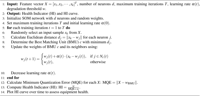
HI Trend Prediction Algorithm

Full size image

Prediction algorithm

    Based on the bearing health indicators established in Chapter 2, this chapter studies the health trend prediction of bearings. Since the health trend of the bearing is monotonically decreasing and irreversible, which is a typical time series process, this chapter considers predicting the health indicators of the bearing at the next moment and subsequent moments from the perspective of time series. Assume that the health indicators of the bearing at the current moment and the previous d moments are: ({H_i}(t),{H_i}(t – 1),ldots ,{H_i}(t-d)), then the health index of the bearing at time (t+1) is ({H_i}(t + 1) = f({H_i}(t),{H_i}(t-1), ldots ,{H_i}(t-d))). Where f represents the prediction model function. It can be seen from formula (20) that this chapter boils down the bearing health prediction problem to the prediction problem of time series data. By selecting an appropriate prediction model, the bearing health index trend can be predicted²⁷.

Normally, the process of model training in the Bi-LSTM network²⁸ requires optimizing the hyperparameters and selecting a set of optimal hyperparameters for the network model to improve the performance of the model. Performance and results. When training a deep Bi-LSTM network, the number of layers and hidden units in the network, as well as the initial learning rate in the network, will affect the training behavior and performance of the network. Choosing the depth of an LSTM network involves balancing speed and accuracy. For example, deeper networks may be more accurate but take longer to train and fit. Therefore, this chapter proposes a Bi-LSTM model hyperparameter optimization method based on Bayesian optimization based on Chapter 2 to further improve the prediction accuracy of the Bi-LSTM model and the generalization ability of the model, and use it for the health trend prediction of bearings are predicted, and the prediction results are compared and analyzed with several other methods.

To take advantage of the outstanding advantages of the Bi-LSTM network in time series, this chapter will study the prediction method based on Bi-LSTM and apply it in the prediction of bearing health indicator trends.

Bayesian optimization algorithm

    Traditionally, experienced domain experts identify optimal sets of hyperparameters, but often produce suboptimal results²⁹. In a variety of applications, Bayesian Optimization (BO) outperforms grid search and random search in hyperparameter tuning, and in some cases outperforms domain experts^29,30. It can effectively find the global optimal solution for unknown functions and complex functions, making it suitable for the automatic tuning process of various algorithms. Compared with traditional optimization algorithms, the BO algorithm can obtain satisfactory results with a smaller number of iterations.

Considering the health index curve constructed in the previous chapter and the use of comprehensive evaluation functions to select degradation characteristics, when predicting the health trend of bearings based on the LSTM network, reasonable LSTM network hyperparameters need to be determined, This chapter proposes a bearing health trend prediction method based on the Bayesian optimized LSTM network method, and optimizes the hyperparameters of the constructed LSTM network.

The hyperparameter optimization problem of the Bi-LSTM deep learning network can be considered as the following optimization problem and solved³¹:

Among them, the hyperparameter combination (X = {{x_1},{x_2}, ldots , {x_n}}), (x_n) is the value of the nth hyperparameter, which can be the number of network layers, the number of hidden units, the initial learning rate, etc.; f(x) is The objective function can be expressed as Mean Max Absolute Error (MMAE), Root Mean Square Error (RMSE), etc. The core of Bayesian optimization is Bayes’ theorem. In Bayesian optimization, we aim to find the minimum of a function a bounded set X value. Bayesian optimization differs from other programs in that it builds a probabilistic model for f(x) and then uses this model to decide where to evaluate the function in x while incorporating uncertainty. The basic principle is to utilize all previously available information rather than simply relying on local gradients and Hessian approximations³². This results in a procedure that can find the minimum of a difficult non-convex function with relatively few computations, but at the cost of performing more computations to determine the next point to try. When computing f(x) is expensive, as it is required to train a machine learning algorithm, then it’s easy to justify some extra computation to make better decisions.

Bayesian optimized Bi-LSTM network model

Bi-LSTM network model

    The characteristic of the LSTM network is to deduce unknown information in the future based on known information in the past. Bi-LSTM takes into account both the past and subsequent information patterns at the predicted moment. Architecturally, BiLSTM includes forward and backward LSTM layers and the inputs from the forward and backward layers are processed simultaneously by the output layer, as shown in Fig. 2. It has been successfully used in character classification annotation, machine reading comprehension, social language sentiment analysis, highway traffic volume prediction, etc.^33,34.

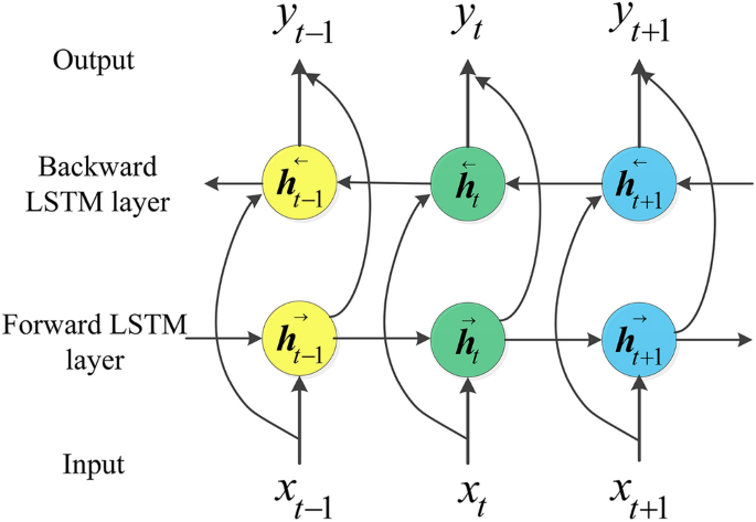
Bi-LSTM model expansion diagram.

Full size image

This article uses adaptive moment estimation (Adam) to optimize the learning rate of the Bi-LSTM network³⁵. It has been proven to be better than stochastic gradient descent with momentum (SGD) and root mean square propagation (RMSProp)³⁶.

Bi-LSTM network hyperparameters

    The hyperparameters involved in the bearing health trend prediction based on the Bayesian optimized BiLSTM network proposed in this article mainly include the number of BiLSTM network layers (BiLSTM Depth), the initial learning rate (Initial Learn Rate), and the number of hidden layer neurons (Num Hidden Units), solver (solver), dropout coefficient (Dropout), number of iterations (epoch), regularization coefficient (Regularization).

The initial learning rate is a very important hyperparameter in the BiLSTM network model³⁷. The initial learning rate is too low and the training time is too long. If the initial learning rate is too high, training may reach suboptimal solutions or diverge. Therefore, it is particularly important to choose a moderate initial learning rate.

The number of iterations indicates the number of iterations of the data set during the model training process. Too many iterations will result in longer training time and overfitting of the model; if the number of iterations is set to too few, the fitting degree of the data will be low, which will affect the performance of the model. Prediction accuracy.

The number of hidden layer neurons is usually determined based on empirical formulas. Increasing the number of hidden units will lead to overfitting of the model and longer training time, and the model will easily fall into local optimality, slowing down the convergence rate of the model. If the number of hidden layer neurons is too small, the model cannot learn enough experience, which will lead to insufficient data fitting.

Using regularization can help avoid overfitting or reduce model errors. This article uses L2 regularization to prevent overfitting. The BiLSTM model cannot have too many layers. The increase in the number of BiLSTM layers will cause the training time and required memory to increase exponentially. When the number of layers exceeds three, the gradient disappearance between layers becomes very obvious.

Bayesian optimization of Bi-LSTM model hyperparameters

    Considering that changes in the number of network layers in BiLSTM will lead to differences in prediction performance, this article needs to set the number of networks as hyperparameters, and BO optimize it. In addition, the hyperparameters of the BiLSTM network need to be optimized, including the initial learning rate, the number of hidden layer neurons, and the L2 regularization coefficient. The remaining hyperparameters are based on experience³⁸.

Based on the Bayesian optimization of BiLSTM network hyperparameters flow chart is shown in the Fig. 3 below.

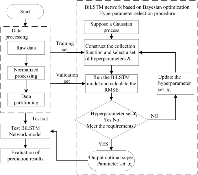
Bayesian optimization of BiLSTM network hyperparameters.

Full size image

The steps for Bayesian optimization of BiLSTM network hyperparameters are as follows:

1. (1)

   According to the range of BiLSTM model hyperparameters, randomly generate an initialization parameter set, input the initialization parameter set into the BiLSTM model and Gaussian model, train the BiLSTM model, and use the loss value output by the objective function to correct the assumed Gaussian model;

2. (2)

   The sampling function constructed using the Gaussian model selects the next set of hyperparameters set (x_i), which is brought into the BiLSTM model for training, obtains the new output value (y_i) of the objective function, and adds ((x_i,y_i)) to the set of samples D, while updating the Gaussian model.

3. (3)

   Determine whether the objective function loss value corresponding to the newly selected hyperparameter set (x_i) meets the requirements. If it does not meet the requirements, add ((x_i,y_i)) to the sample set D and jump to Go to the second step and continue to execute the Bayesian optimization algorithm; if the requirements are met, the Bayesian optimization algorithm is terminated, and the current hyperparameter combination and the loss value of the corresponding BiLSTM model’s objective function are output at the same time (y_i).

    To verify the generalizability of the health assessment method and process of the bearing performance degradation process proposed above, PHM2012 bearing data was selected as experimental data for verification³⁹.

Data description

    Loading different loads can simulate different operating conditions, PRONOSTIA experimental platform (Fig. 4) accelerated degradation experiments on rolling bearings can obtain measured data during the entire life cycle, this data set can be used for failure analysis, condition assessment, remaining life prediction, etc. of rolling bearings. The details of the PHM2012 data set are shown in Table 3. The data set includes 3 working conditions. The data set under each working condition includes vibration signals and temperature signals. The vibration signal is divided into horizontal and vertical vibration values. The sampling frequency of the data is 25.6 kHz, the sampling time is 0.1 s, and it is collected every 10 s.

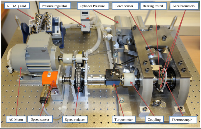
PRONOSTIA experimental platform.

Full size image

This article selects the Bearing1_1 to Bearing1_7 data set under working condition 1 and uses the vibration value in the horizontal direction for testing. Bearing1_1 and Bearing1_2 are training sets, which contain data from the entire life cycle from the initial healthy state to the degraded failure state; Bearing1_3- Bearing1_7 are test sets, which only contain partial shear data from the initial healthy state to the degraded state. The original vibration signals in the horizontal direction from Bearing1_1 to Bearing1_7 are shown in Fig. 5.

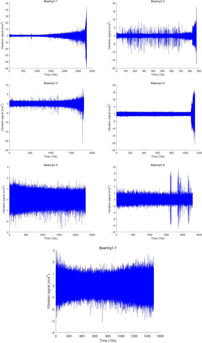
Bearing1_1-Bearing1_7 original vibration signal under working condition 1.

Full size image

Feature selection

    Calculate the 36-dimensional degradation characteristics of Bearing1_1 to Bearing1_7 based on the time domain, frequency domain, and time-frequency domain features⁴⁰ in Chapter 1. Since Bearing1_1 and Bearing1_2 are training sets, including data of the entire life cycle, four evaluation indicators of monotonicity, correlation, robustness, and predictability of the 36-dimensional degradation characteristics of Bearing1_1 and Bearing1_2 are obtained based on relevant calculations, as shown in Fig. 6 shown.

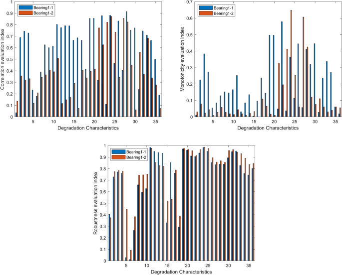
Monotonicity, correlation, and robustness evaluation indicators of Bearing1_1 and Bearing1_2.

Full size image

The monotonicity, correlation, and robustness evaluation indexes of the 36-dimensional degradation features of Bearing1_1 and Bearing1_2 are averaged respectively, and finally, the comprehensive evaluation function constructed according to Eq. (14) is used for feature selection. Similarly, let (lambda _1=0.5), (lambda _2=0.25), (lambda _3=0.25,) (lambda _4=0), and select the features with a comprehensive evaluation index (J>0.4). Then the final selected degradation features are (P_3) square root amplitude, (P_{11}) waveform index, (P_{19}) amplitude skewness index, (P_{20}) amplitude craggy-ness index, (P_{21}) center frequency, (P_{22}) frequency standard deviation, (P_{23}) root-mean-square frequency, (P_{24}) frequency variance, and (P_{25}) root-mean-square frequency, (P_{26}) frequency combination feature, (P_{27}) frequency domain frequency skewness, (P_{28}) frequency domain frequency crag, (P_{29}) square root ratio, P30IMF energy1, P33IMF energy3 total 15-dimensional features⁴¹.

Construct a health indicator curve

    Using the content in Section “Self-organizing feature mapping network”, select the first 100 sets of feature values as the training set to train the SOM network. Set the number of SOM network neurons to 15, consistent with the selected degradation feature vector dimension, and the weight dimension to (5 times 5); set the initial learning rate to 0.9, and the number of training times to 500. Input the degraded feature values of the training set and test set into the trained SOM network, calculate the corresponding MQE, and perform sliding average processing with a window size of 10, as shown in Fig. 7. In this example, the maximum value of MQEofBearing1_1 and bearing1_2 is taken as 30. Finally, the HI curve of each bearing⁴² is obtained according to Eqs. (4–5), as shown in Fig. 8 shown. It can be seen from the figure that during the operation of the bearing, its health indicators are constantly changing, and the health indicators reflect the operating performance of the bearing at the current moment.

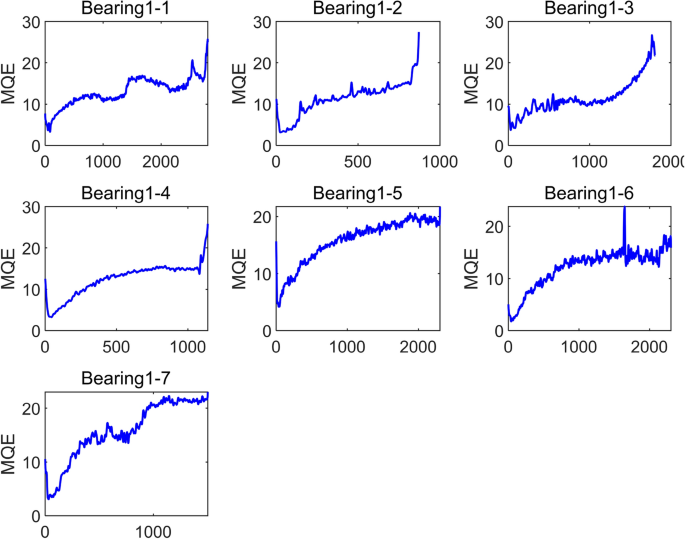
MQE curve of Bearing1_1-Bearing1_7 under working condition 1.

Full size image

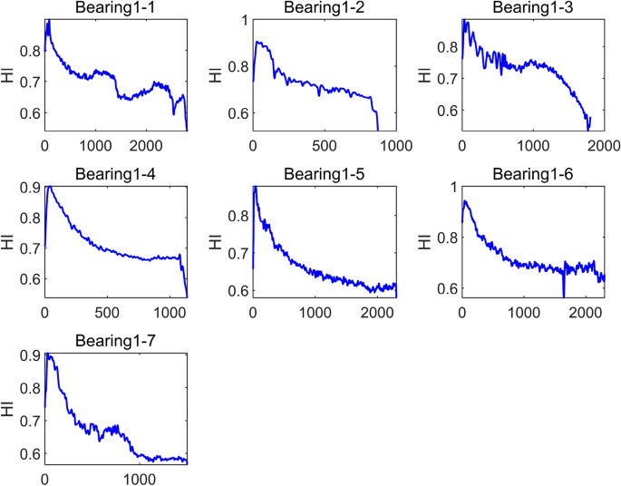
HI curve of Bearing1_1-Bearing1_7 under working condition 1.

Full size image

Because Bearing1_1 and Bearing1_2 are training sets, with data from the initial operating state to degradation failure, and Bearing1_3 to Bearing1_7 are test sets, with only partial shear data, that is, the four bearings from Bearing1_3 to Bearing1_7 have not yet completely failed. Status, as can be seen from Fig. 9, the health index of Bearing1_1 when it fails is 0.522312, the health index of Bearing1_2, when it fails, is 0.521831, and the final health indexes of Bearing1_3 to Bearing1_7 are all smaller than these two values. Taking Bearing1_5 as an example, its final health index is 0.580008, which proves that the health index of the structure is reasonable, and can reflect the health status of the test bearing⁴³. It can be seen from the changes in the health indicators in the figure that the bearings have gone through the health stage of initial operation during actual operation, and the performance degradation stage is the final failure stage⁴⁴.

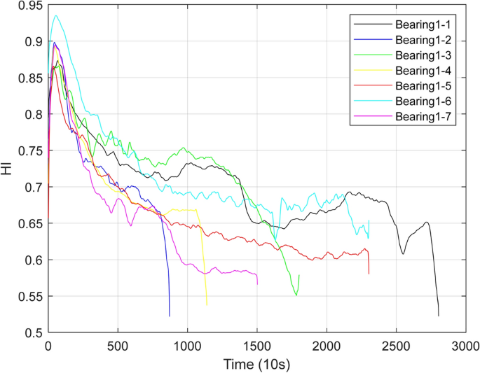
HI curve of Bearing1_1-Bearing1_7 under working condition 1.

Full size image

Health status assessment

    To better distinguish the stages of bearing performance degradation, provide a scientific basis for the subsequent maintenance and replacement plan of wind turbine bearings, and ensure the safe and reliable operation of wind turbines. This article observes and summarizes the changes in health indicators of the above seven bearings, and maps the quantitative evaluation of health indicators with the qualitative evaluation levels of operating status. The health status of the bearings can be divided into 3 levels⁴⁵: when the health index is [0.8, 1] When it is within the range, the bearing is in good health and is in healthy operation; when the health index is [0.65, 0.8] When the health index is less than 0.65, the bearing’s operating performance has shown certain signs of abnormality, and its health status has seriously degraded. On-site operation and maintenance engineers need to focus on the bearing’s health. Operating status, taking corresponding adjustment plans promptly, formulating relevant maintenance measures, and even replacing bearings with severely degraded performance⁴⁶. Table 4 shows the classification of bearing health index levels and corresponding operating status.

Health indicator trend prediction

Data description

    This paper selects the time domain, frequency domain, and time-frequency domain characteristic values of Bearing1_1 to Bearing1_7 under working condition 1, and performs trend prediction on health indicators.

Assume that a health indicator time series of the bearing is (X = [{x_1},{x_2}, ldots ,{x_n}]), which contains n time step data. The PRONOSTIA experimental platform samples every 10 seconds. We assume that the first d previous health indicator values may have a periodic impact on the current predicted output value. The first d values can be expressed as a set, set (L = [{D_1},{D_2}, ldots ,{D_d}]), where (d < n). By adding the set L, the original set of time series X can be transformed into a matrix ({X_{re}})⁴⁷ of dimension (d times n) as shown in Eq. (21) below⁴⁸:

In this way, the matrix (X_{re}) can correspond to the original time series X in the time series dimension. Combining the matrix (X_{re}) with the predicted value at the next moment, the new matrix (X_{pre}) with dimension ((d+1) times n) is as shown in the following Eq. (22)

The first d rows are the inputs of the BO-BiLSTM network model, and the last row is the target time series that needs to be predicted⁴⁹. According to the above method, in each time step prediction, the data of the previous d time steps can be used to predict the current data. Therefore, using the (X_{re}) matrix to predict the X target time series, the relationship between the previous value and the predicted value can be detected.

Parameter settings

    In this verification, the basic structure of the BiLSTM model consists of a hidden layer, a fully connected layer, and an output layer⁵⁰. To prevent overfitting, a dropout layer is set (dropout) coefficient is 0.5, batch size (batch-size) is set to 64, and the number of iterations (epoch) is set to 400. Select the adaptive moment estimation (Adam) solver, use the linear rectified function (Rectified Linear Unit, ReLU) as the activation function, select the root mean square error (Root mean square error, RMSE) as the target loss function, BO-BiLSTM network, the maximum number of iterations of Bayesian optimization is 60⁵¹. Other hyperparameters that need to be optimized and their value ranges are shown in Table 5 below:

Prediction performance evaluation indicators

    This section uses five commonly used statistical indicators, namely mean absolute error (MAE), root mean square error (RMSE), mean absolute percentage error, mean absolute percentage error (MAPE), and coefficient of determination (R^2) (coefficient of determination) to comprehensively evaluate the relevant model⁵², as shown in Eqs. (23)–(26). In principle, the smaller the MAE, RMSE, and MAPE, the smaller the error between the actual value and the predicted value. The closer (R^2) is to 1, the more accurate the prediction result will be. Here, (y_i) and (hat{y}_i) represent the actual value and the predicted value respectively, (bar{y}_i) represents the average of (y_i), and N is the number of actual data points.

In this verification, the health indicator data of Bearing1-1 was divided into a training set, verification set, and test set in a ratio of 8:1:1. To facilitate the experimental comparison of different algorithms, the basic parameters of LSTM, BiLSTM, and BO-BiLSTM are set to be consistent, that is, the number of network layers is set to 1 layer, dropout is 0.5, batch-size is 64, epoch is 400, and the number of neurons is 100, the initial learning rate is 0.05, and the L2 regularization coefficient is 0.0001. Input the Bayesian optimized BiLSTM network hyperparameters into the model to obtain the BO-BiLSTM prediction results, and compare them with the traditional LSTM and BiLSTM model prediction results to verify that the Bayesian optimization algorithm can obtain a hyperparameter combination that makes the BiLSTM model prediction accuracy higher.

After the Bayesian optimization hyperparameter process in Section “Bayesian optimized Bi-LSTM network model”, the optimal hyperparameter combination is obtained as shown in Table 6 below:

Bring the above optimized hyperparameter combination into the BO-BiLSTM model⁵³, and use the first 60 moments to predict the health index value of Bearing1-1 at the next moment. The prediction results are shown in Fig. 5, 6, and 7 below. The first 2254 data in the figure are training data. The training data are used to obtain the hyperparameters of the BO-BiLSTM network model, and then the last 549 test data are used to test the BO-BiLSTM network model. The red curve in Fig. 10 represents the true value of the test data, and the blue curve represents the predicted value of the test data. It can be seen from Fig. 11 that the blue curve and the red curve overlap, which shows that the bearing Bearing1-1 The prediction of health indicators is relatively accurate⁵⁴.

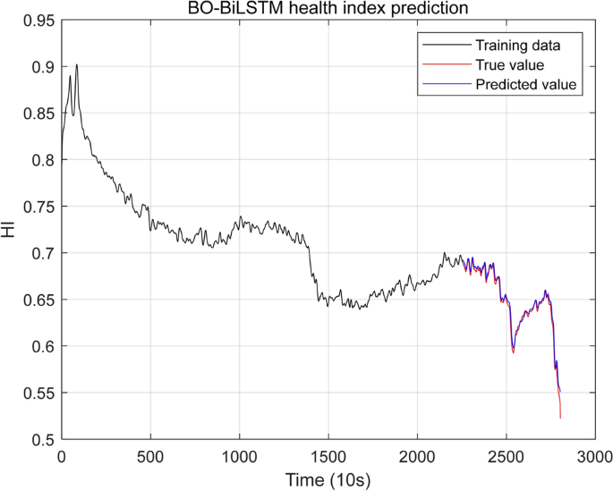
BO-BiLSTM health indicator prediction results.

Full size image

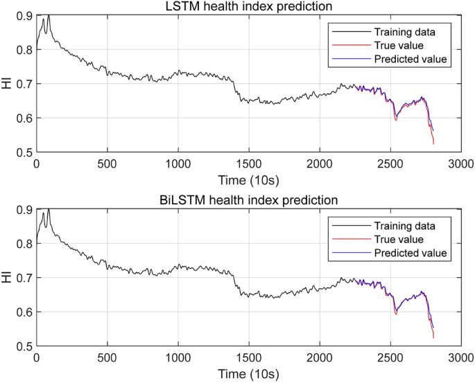
LSTM and BiLSTM health indicator prediction results.

Full size image

At the same time, this section also uses the LSTM network model and the BiLSTM network model to predict the degradation trend of the health indicators of the bearing Bearing1-1. The prediction results are shown in Fig. 11. It can be seen from this figure that the predicted value of the LSTM network model deviates significantly from the true value. Compared with the LSTM network, the prediction results of the BiLSTM network are relatively accurate, but compared with the BO-BiLSTM network, its prediction accuracy is still slightly insufficient.

In order to further illustrate that the BO-BiLSTM network model has higher prediction accuracy, this section compares the prediction results of LSTM, BiLSTM, and BO-BiLSTM networks, as shown in Fig. 12 below. According to formulas (23)–(26), the evaluation indicators of the predicted values and true values of each network model are calculated, as shown in Table 7 below.

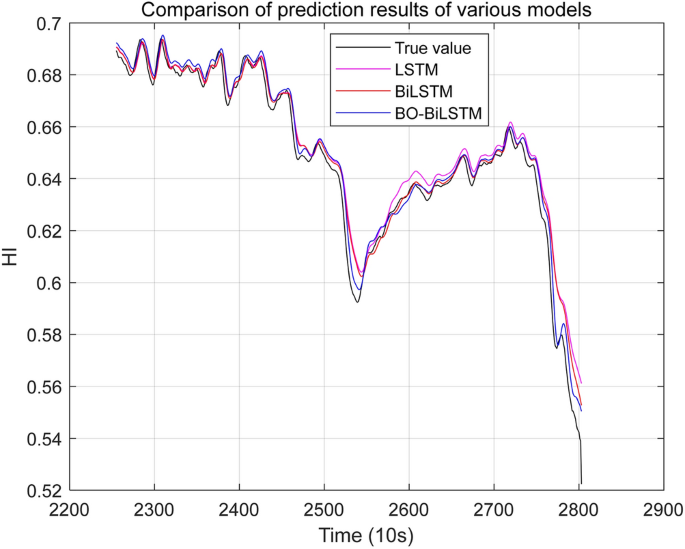
Comparison of health indicator prediction results of various network models.

Full size image

From the prediction performance evaluation indicators listed in Table 7, it can be clearly seen that for the same bearing Bearings1-1, the BO-BiLSTM network model has the lowest RMSE, MAE, and MAPE, and the best result is obtained by using the BO-BiLSTM network model to predict health indicators.

    This paper proposes a method for constructing a HI curve by combining a comprehensive evaluation function with a self-organizing neural network to assess the health status of wind turbines and predict the health degradation trend of wind turbine bearings using the BO-BiLSTM model.

1. 1.

   For the extracted high-dimensional degradation features, the comprehensive evaluation function can eliminate features that do not reflect the degradation process of wind turbine bearings and those with poor performance in reflecting the degradation process.

2. 2.

   A single time-frequency domain degradation feature hardly reflects the degradation trend of wind turbine bearings. The HI curve generated by fusing the selected degradation features using the SOM algorithm can more accurately reflect the health status of the high-speed shaft bearings.

3. 3.

   Given the complex structure of the Bi-LSTM network and the difficulty in hyperparameter optimization, the Bayesian optimization algorithm is used to find the global optimal hyperparameters for the Bi-LSTM network.

4. 4.

   The BO-BiLSTM model is utilized to predict the degradation trend of wind turbine bearings. Under the same hyperparameter settings, the prediction results of the BO-BiLSTM model are superior to those of the BO-LSTM model.

5. 5.

   Based on the constructed HI curve, further prediction of the remaining life of wind turbine bearings can be carried out.

6. 6.

   Trend prediction of the health status of wind turbines can provide theoretical support for the subsequent scientific and rational maintenance plans of wind farms.