Hierarchical and distinct biological motion processing in macaque visual cortical areas MT and MST

Introduction
Perceiving the movement of other living creatures is of survival importance for many species. Humans and other primates can readily recognize body movements and perceive biological motion (BM) from even simplified kinematic information of a dozen point-lights attached to the joints of an actor1. It is generally accepted that both form and motion information contribute to BM recognition2, but motion cues seem to be more critical3,4. BM perception from the point-light display has two hallmark characteristics: one is the inversion effect, that is, turning the display upside-down severely impairs BM recognition5,6, and the other is the scrambling effect, i.e., BM recognition is completely lost when individual point-lights are spatially scrambled such that the form information is destroyed7. Correspondingly, a preferential neural representation of intact upright BM (relative to inverted or scrambled BM) is often regarded as a marker of BM-specific processing in the brain8.
BM perception generally involves a network of distributed cortical and subcortical brain structures specialized for processing socially relevant information8,9,10. In particular, the posterior superior temporal sulcus (pSTS) is the region most prominently associated with BM processing8,11. Neuroimaging studies have well documented that the pSTS is more active when subjects view intact upright BM than scrambled or inverted BM12,13,14. Yet, on a more fine-grained scale, the pSTS contains two important subregions particularly relevant for the analysis of visual motion signals15,16. One subregion is the middle temporal area (MT), a key motion-sensitive area in the primate visual cortex where neurons respond selectively to simple translational motion in a direction-selective manner17,18,19. The second subregion is the adjacent medial superior temporal area (MST). MST receives direct feedforward input from MT20 and responds selectively to more complex motion patterns such as optic flow defined by expansion and rotation21,22. Since BM stimuli likely activate neurons in both MT and MST, an important question to ask is, whether BM-specific processing is established in area MST or is determined earlier in area MT. So far, our understanding of BM computation at the single-cell and neural circuit levels within pSTS is still limited.
Only a few single-cell electrophysiological studies have attempted to address the visual recognition of biological movements (for action-based movement recognition, see a plethora of mirror neuron studies in recent reviews23,24). Early studies in monkeys have found that neurons in the superior temporal polysensory (STP) area respond selectively to displays of body movements25. As a polysensory brain area, STP sits at the anterior section of the STS (also known as aSTS), responsible for integrating information from upstream areas such as the posterior section of the superior temporal sulcus (pSTS) and the fundus of the superior temporal sulcus (FST)26,27. Anatomically, the pSTS is the first stage of BM processing, which is then fed to area FST and subsequently integrated within area STP. While it certainly remains to be understood how biological motion is hierarchically computed and represented along these posterior-anterior STS gradients, the current study focused exclusively on the posterior portion of this circuit. We aim to investigate how individual neurons and neural circuits within pSTS support BM recognition.
We addressed these questions with neurophysiological recordings in awake-behaving monkeys and neural network modeling. We first examined the neuronal correlates of BM processing in MT and MST respectively. We then built a neural network model trained to replicate these neurophysiological data and, more importantly, to shed connectivity insights on how these two pSTS subregions might interact to achieve BM-specific computations in the primate brain.
Results
Neuronal datasets and analysis
We trained three macaque monkeys to view BM stimuli and recorded single-cell spiking activity from area MT and MST (Fig. 1a, b), using standard extracellular techniques (see “Methods”). The full datasets consisted of 129 MT neurons and 228 MST neurons from three monkeys. Since neuronal responses were similar between monkeys, we pooled them together for data analysis and presentation. Note that the MST dataset has been analyzed previously in our recent paper28. The current study re-analyzed the same MST dataset and a new MT dataset collected under identical stimulus conditions. We sought to quantitatively compare stimulus selectivity and BM-specific processing across these two pSTS subregions.

a Trial sequence. In each trial, monkeys were required to maintain fixation on a small red dot while viewing point-light animations depicting various BM stimuli. b Schematics of the extracellular recordings in two pSTS subregions (MT and MST). c BM stimuli portray BM walking in different directions (left vs. right), orientations (upright vs. inverted), and forms (intact vs. scrambled). (b) was adapted from a cartoon image deposited at SciDraw by Andrea Colins Rodriguez (https://doi.org/10.5281/zenodo.4662738), with additional graphic elements added by the first author of this study.
The task for the monkeys was to passively view point-light displays while maintaining gaze fixation at the center of the screen. We manipulated the walking direction (left vs. right), body orientation (upright vs. inverted), and body form (intact vs. scrambled) of BM stimuli (Fig. 1c). Contrasting neuronal responses within each comparison allowed us to assess the selectivity (or detectability) strength of individual neurons to these BM features. Given the rhythmic nature of BM stimuli (with a walking cycle of 2 Hz), the elicited neuronal responses were also not stationary but rather oscillatory during stimulus presentation. Following previous conventions28,29,30, we applied the spectral analysis to the spike density response to derive a so-called “modulation index” (MI) as a measure of BM-modulated neural response (see “Methods”). These MIs were subsequently contrasted across stimulus conditions (e.g., left vs. right) to obtain the detectability index (DI). DI represented the ability of each neuron to distinguish the BM feature under comparison (e.g., walking directions).
MT and MST cells exhibit comparable and balanced BM direction selectivity
Direction selectivity is the most prominent feature of neurons in motion-sensitive areas. Similar to our previous findings in MST, responses of MT neurons were also dynamically modulated by BM stimuli, and these modulations were BM direction-dependent. As can be seen from two example MT neurons (Fig. 2a), the upper neuron exhibited larger modulation effects when BM walking to the right (MI = 0.82), relative to when BM walking to the left (MI = 0.39). In other words, this neuron preferred right-walking BM. In contrast, the neuron in the lower panel preferred left-walking BM (MI = 2.22 and 0.85, respectively).
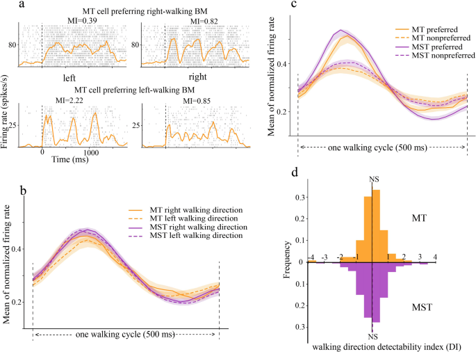
a The raster and spike density responses of two example MT neurons to BM walking directions. The modulation index (MI) showed directional preferences. b Normalized population responses of MT (orange) and MST (purple) neurons to left-walking (dashed) and right-walking (solid) BM. c The same as in (b) but sorted into preferred and non-preferred directions. d The distribution of direction DI in MT (upper) and MST (lower). The vertical dashed lines mark the mean direction DI in each area.
At the population level, the direction preference for left vs. right was balanced and comparable between areas MT and MST. To reveal the dynamic coding of walking directions, we calculated the mean normalized firing rates in one walking cycle (0–500 ms relative to stimulus onset). We found that the mean population responses induced by right-walking and left-walking BM stimuli overlapped, in both MT and MST areas (Fig. 2b). However, the mean population responses sorted by preferred vs. non-preferred directions showed clear separations, indicating a capability of discriminating BM directions for neurons in these two brain areas (Fig. 2c). To more quantitatively compare BM direction selectivity across areas, we plotted the distribution of direction DIs for each brain area (Fig. 2d). First, the mean direction DIs in MT and MST did not differ significantly from zero (MT: mean = 0.02, t(128) = 0.36, p = 0.72, one-sample t-test; MST: mean = 0.04, t(227) = 0.49, p = 0.69, one-sample t-test). This again indicated that the ability to detect right-walking and left-walking BMs was balanced in both areas. Second, the mean direction DIs did not differ between MT and MST (Welch’s two-sided t-test: t = 1.08, p = 0.87), suggesting that BM direction coding was equally strong in these two visual areas.
MST but not MT cells show BM-specific processing—biased form and inversion selectivity
BM recognition has two defining characteristics, the inversion effect, i.e., severely impaired recognition of inverted BM, and the scrambling effect, i.e., entirely disrupted recognition of scrambled BM. Hence, biased neuronal selectivity for form and inversion could be regarded as an indication of BM-specific processing at the neural level. In this section, we will examine the form and inversion selectivity in MT and MST respectively, testing whether these selectivity are biased. This will help us to determine whether BM-specific processing is established in area MST or occurs early in area MT.
Form selectivity could be estimated by comparing neuronal responses evoked by intact and scrambled BM. Figure 3a shows the spiking responses of two example MT neurons. We can see that the MT neuron at the top exhibited greater modulation in response to intact BM (MI = 1.46) than scrambled BM (MI = 0.79). In contrast, the MT neuron at the bottom was also strongly modulated by BM, but its modulation showed a preference for the scrambled BM (MI = 2.45) relative to the intact BM (MI = 1.1). At the population level, the form selectivity was balanced in area MT but biased in area MST toward preferring the intact BM (Fig. 3b–d). This can be observed from two analyses. First, the population mean responses overlapped in MT but diverged in MST (Fig. 3b), with the intact BM evoking stronger responses relative to the scrambled BM. This indicated that while MT cells had a balanced preference for intact and scrambled BM, MST cells showed a preferential representation of intact BM than scrambled BM. Second, this claim was also supported by the quantitative form DI distribution analysis (Fig. 3d). The mean form DI in area MT was close to zero (mean = 0.04, t(128) = 0.67, p = 0.51, one-sample t-test), suggesting that while individual MT neuron responded differently to intact and scrambled BM (Fig. 3c), their preference at the population level was balanced. In comparison, the mean form DI in area MST was significantly biased toward preferring intact BM (mean = 0.39, t(227) = 7.69, p = 4.39 × 10⁻¹³, one-sample t-test). The difference in form selectivity between MT and MST was also verified directly (t = 4.5, p = 9.65 × 10⁻⁶, Welch’s two-sided t-test).
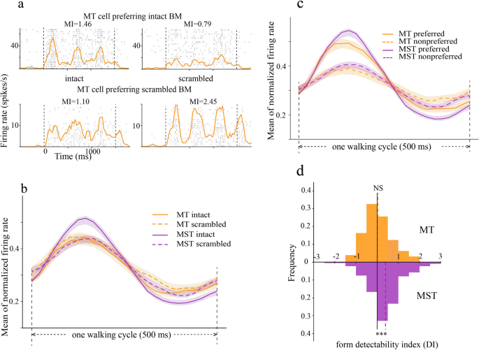
a The raster and spike density responses of two example MT neurons to intact and scrambled BM. The top neuron preferred intact BM while the bottom neuron preferred scrambled BM. b Normalized population responses of MT (orange) and MST (purple) neurons to intact (solid) and scrambled (dashed) BM. c The same as in (b) but sorted into preferred and non-preferred forms. d The distribution of form DI in MT (upper) and MST (lower). The vertical dashed lines mark the mean form DI in each area. ***p < 0.001.
We performed similar analyses for the inversion selectivity and found that MST but no MT cells showed biased inversion selectivity. Figure 4a depicts the spiking responses of two example MT neurons to upright and inverted BM. The top MT neuron showed larger modulated responses to inverted BM (MI = 1.6) than upright BM (M = 0.65), indicating a preference for inverted BM. Oppositely, the bottom MT neuron preferred upright BM (MI = 2.28) relative to inverted BM (MI = 1.07). At the population level, the preference for upright vs. inverted BM was balanced in MT but was biased toward preferring upright BM in area MST (Fig. 4b–d). First, as a visual inspection of the population mean responses (Fig. 4b), upright and inverted BM elicited similar MT responses. Meanwhile, upright BM elicited larger responses than inverted BM in MST. Second, the neural preference for upright BM in area MST but not MT could also be observed quantitatively from the inversion DI distributions (Fig. 4d). The mean inversion DI in area MST was significantly biased toward preferring upright BM (mean = 0.18, t(227) = 2.85, p = 0.005, one-sample t-test). In contrast, the mean inversion DI in area MT was indistinguishable from zero, indicating balanced neural preference (mean = 0.07, t(128) = 1.1, p = 0.27, one-sample t-test).
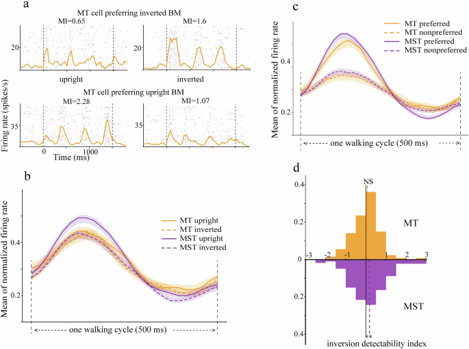
a The raster and spike density responses of two example MT neurons to upright and inverted BM. The top neuron preferred upright BM while the bottom neuron preferred inverted BM. b Normalized population responses of MT (orange) and MST (purple) neurons to upright (solid) and inverted (dashed) BM. c The same as in (b) but sorted into preferred and non-preferred body orientation. d The distribution of inversion DI in MT (upper) and MST (lower). The vertical dashed lines mark the mean inversion DI in each area. **p < 0.01.
Independent BM encodings in area MST
To sum up, we have so far characterized and compared the selectivity responses of MT and MST neurons to BM stimuli. Our results revealed that, while cells in both brain areas were selective for each of the BM features, cells in MST but not MT showed BM-specific processing. In other words, MST cells had biased form and inversion selectivity, preferring intact (vs. scrambled) and upright (vs. inverted) BM. It should be noted that the biased form and inversion selectivity in MST could not be trivially explained by biased sampling in the recorded population for two reasons. First, as we showed already in the previous section, the direction selectivity in area MST (and in area MT as well) was perfectly balanced between left- and right-walking directions (Fig. 2b–d), arguing against biased sampling. Second, the Pearson correlation analysis revealed that neither the form selectivity nor the inversion selectivity in MST was correlated with its direction selectivity (Inversion DI vs. direction DI: r(226) = −0.07, p = 0.28; Form DI vs. direction DI: r(226) = 0.01, p = 0.83). This suggested that these biased encodings in MST reflected neural features independent from the basic motion direction representations, and should be better interpreted as serving the neural correlates of the inversion and scrambling effects observed behaviorally during BM recognition.
It is also worth noting that, the two biased encodings in MST, i.e., the BM-specific processing in the form and inversion selectivity, were also independent from each other (r(226) = 0.02, p = 0.75, Pearson correlation). These independent representations of BM features in area MST suggested that they were probably encoded in distinct neural subpopulations or in shared neural population but through distinct computations. Either way, these independent encodings do not refute the idea of BM-specific processing in MST. Meanwhile, we should point out that the neural bias being larger in the form selectivity than in the inversion selectivity was not unexpected. In fact, it aligned well with their effect size differences at the behavioral level. Psychophysical studies have shown that scrambling does more damage to BM recognition than inversion (entirely lost by scrambling vs. partially impaired by inversion). It is hence reassuring for us to observe neural effect size differences, i.e., relatively large form bias but smaller inversion bias in the neurophysiological data.
A spiking neural network model replicated neurophysiological data and implicated connectivity patterns underlying the emergence of BM-specific processing in MST
The distinct BM-specific processing in MST but not MT begs the question of how a balanced encoding in area MT would lead to biased representation in MST who receives direct input from MT? or how the two areas might interact to give rise to BM-specific, biased representation in the brain. We addressed these questions with neural network modeling in this section.
To reveal the computational mechanisms underlying the distinct BM processing in MT and MST, we used the recorded neurophysiological data to train a two-layered spiking neural network (SNN) model31, mimicking feedforward spike train transmission from MT to MST (Fig. 5a, b). In brief, The SNN consisted of an input MT layer and an output MST layer that were fully connected. The number of MT and MST neurons and their neuron types matched the electrophysiological data. The spike trains of the collected 129 MT neurons during stimulus presentation period (0–1500 ms, binned at 10 ms in each epoch) were provided as the inputs to the model. On a given trial, each MT neuron i (i = 1, 2, 3,…129) transmits a spike train ({{{rm{S}}}}_{{{rm{i}}}}^{{{rm{MT}}}}) to each output MST neuron j (j = 1, 2, 3, …, 168), inducing a postsynaptic potential ϵi(t) on MST neuron j. The membrane voltage μj(t) of MST neuron j is the weighted sum of wji·ϵi(t) from all MT neurons. If the μj(t) exceeds a threshold θ (red dotted line), the MST neuron j will emit an output spike (({{{rm{S}}}}_{{{rm{j}}}}^{{{rm{a}}}})) and enter the refractory period. The initial connectivity weights wji between MT and MST neurons were randomly and were updated during training. After training, the model reproduced the spike trains of the collected 168 BM-selective MST neurons under each stimulus condition.
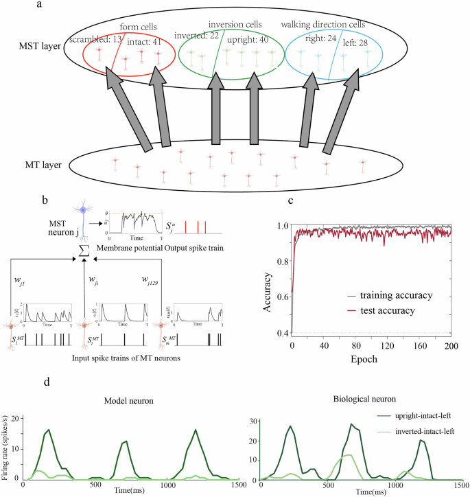
a Model architecture. The two-layered spiking neural network model consisted of an input MT layer and an output MST layer. b Each MT neuron i transmits spike trains ({S}_{i}^{{MT}}) to an output MST neuron j, inducing the postsynaptic potential ϵi(t) on MST neuron j. The membrane voltage μj(t) of MST neuron j is the sum of wji·ϵi(t) for all MT neurons. The MST neuron j will emit an output spike (({S}_{j}^{a})) if the μj(t) exceeds a threshold θ (red dotted line). c The training and test accuracy of the model. d The responses of a model MST neuron and a biological MST neuron were selective for upright BM.
As shown previously, the recorded 168 MST neurons were classified into form neurons, inversion neurons, and walking direction neurons based on their BM selectivity. Then according to neural preference, each neuron type can be further divided into two opposing subtypes (e.g., intact-preferring form cell, scramble-preferred form cell), resulting in a total of six pools of MST neurons: intact-preferred (N = 41), scramble-preferred (N = 13), left-preferred (N = 28), right-preferred (N = 24), upright-preferred (N = 40), and inverted-preferred (N = 22). The model employs a winner-takes-all strategy to determine which MST neuron pool responds most strongly to the stimulus. For example, when a BM stimulus carrying three features (e.g., “intact-upright-left”) was fed into the SNN network, MST neurons in the three target pools (“intact”, “upright”, “left”) were regarded as the target neurons, while those in the non-target populations (“scramble”, “inverted” and “right”) were designated as the non-target neurons. Each non-target neuron should not respond to the motion stimulus and remain silent throughout the simulation. Each target neuron started with randomly generated spike trains which, through weight updating, evolved into the actual spike trains of biological MST neurons in the target pools.
We used the tempotron learning rule to modify the synaptic weights, minimizing a cost function that measures the amount of timing deviations between the actual and desired output spikes32. In an iterative learning scheme, synaptic weights were updated (either increasing or decreasing) by an amount proportional to the cost at each iteration (see “Methods”). The output of the model was expected to reproduce the recorded MST responses after training. To evaluate the performance of model output, we computed the accuracy as a measure of similarity between biological and model MST neuron pools using Hamming distance (see “Methods”). The training and test accuracy were computed at every time epoch. The neurophysiological responses of MT and MST neurons were split across trials, such that the spike trains of 75% of the trials were used for the training process and the remaining 25% of the trials for the test process (cross-validation). It can be observed that the SNN model learned quickly (Fig. 5c). The training accuracy can be up to 99.7%, and the test accuracy can be up to 98.3%, indicating that the MST population had successfully reproduced the desired output spike trains. This means after training, the spike density responses and the selectivity of model MST neurons resembled those of biological MST neurons. As an illustration, Fig. 5d plotted the spiking responses of a model MST neuron (left panel) and a biological MST neuron (right panel). The Pearson correlation analysis indicated that the model neuron and the biological neuron had very similar response profiles (Upright-intact-left: R2 = 0.82, p = 5.8 × 10⁻²⁰; Inverted-intact-left: R2 = 0.35, p = 2.4 × 10⁻⁷), and both of them were inversion-selective and preferred upright BM.
The connectivity weights between MT and MST neuron populations were completely random before training, and the SNN could not perform the BM recognition task. Yet, after training, the model replicated neurophysiological MST responses based on the recorded MT spike train inputs. We hypothesized that the MT-MST connectivity has formed a certain pattern or structure, giving rise to BM-specific processing. We thus examined whether MT neurons projecting to distinct MST cell types would show differences in their basic properties, in responding to the conventional non-biological motion (linear motion and optic flow).
In the trained model, some MT neurons are more densely connected to a type of MST neurons than others. For example, there is an MT neuron projecting to 34 intact-preferred neurons, 1 scramble-preferred neuron, 23 right-walking preferred neurons, 21 left-walking preferred neurons, 8 upright-preferred neurons, and 22 inverted-preferred neurons. If an MT neuron has projection connections to at least half of the MST neurons in a certain type, it is classified as an MT neuron projecting heavily to that type of MST neuron. For the example MT neuron described above, it projected heavily to intact (34/41), left (21/28), right (23/24), and inverted (22/22) preferred MST neurons, but sparsely to scrambled (1/13) or upright (8/40) preferred neurons. Through this classification criterion, we found that the number of MT neurons that project heavily to intact-, scrambled-, upright-, inverted-, rightward- and leftward-preferring MST neurons are 43, 41, 48, 45, 52, and 42, respectively. In the following, we quantified the basic motion selectivity of these 6 pools of MT neurons that projected preferentially to each type of MST cells (3 BM features × 2 preference).
Figure 6a–c plotted the linear motion selectivity and nonlinear optic flow selectivity for each pool of these MT neurons. For MT cells that projected heavily to MST direction cells (Fig. 6c), their linear selectivity strengths were significantly larger than their nonlinear selectivity strengths (rightward-preferring: t(51) = 2.96, p = 0.005; leftward-preferring: t(41) = 2.05, p = 0.047, paired t-test). Similar observations can be made for MT cells that projected heavily to MST inversion cells (Fig. 6b, upright-preferring: t(47) = 4.23, p = 0.0001; inverted-preferring: t(44) = 2.33, p = 0.024, paired t-test). These observations were expected since MT neurons are well known for their sensitivity to simple linear translational motion as compared to more complex motion patterns. For MT cells that projected to MST form cells, their selectivity properties for linear and nonlinear motions diverged depending on their specific form preference (Fig. 6a). MT neurons preferentially connected with scramble-preferring form cells again showed stronger linear selectivity than nonlinear selectivity (right panel, t(40) = 4.3, p = 0.0001, paired t-test). In contrast, MT neurons preferentially connected with intact-preferring form cells showed similar levels of linear and nonlinear selectivity (left panel, t(42) = 1.43, p = 0.16, paired t-test). In other words, relative to other cell types, MST intact-preferring form cells received considerably more information from nonlinear optic flow selective MT neurons.
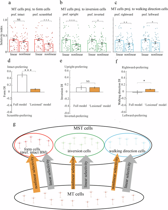
a–c The mean linear motion selectivity and nonlinear optic flow selectivity of MT neurons projected heavily to MST form cells (intact- or scramble-preferring), inversion cells (upright- or inverted-preferring), and direction cells (leftward- or rightward-preferring). Error bars indicate SEM. d–f The impact of removing nonlinear optic flow selective MT neurons in the model: the form selectivity was dramatically impaired while the inversion and direction selectivity were relatively preserved. g The schematic illustration of preferential projection of nonlinear optic flow selective MT neurons to MST form cells (orange arrows), and preferential projection of linear motion selective MT neurons to MST inversion and direction cells (gray arrows).
The connectivity pattern implicated from the model suggested that, while linear motion selective MT neurons projected to each MST cell type equally in an undifferentiated manner, nonlinear optic flow selective MT neurons projected preferentially to MST intact-preferring form cells (Fig. 6g). It seemed that the nonlinear selectivity in the MT population was the critical driving force for form selectivity in area MST. We tested this idea directly with an “ablation” experiment in the model. The reasoning behind was, if nonlinear selectivity in MT plays a critical role in shaping form selectivity in MST, then “lesioning” nonlinear selective MT neurons would impair mainly the form selectivity in MST while leaving the inversion and direction selectivity relatively intact.
In the ablation experiment, we first trained the model with the full MT-MST connectivity as we did previously, we then “lesioned” the model by removing MT neurons whose rotation or radiation selectivity index was greater than 0.33 (i.e., when responding to optic flow, the preferred response was twice as large as the non-preferred response). This allowed us to assess the form, inversion and direction selectivity of the simulated MST population before and after lesion (Fig. 6d–f). There were two noteworthy observations. First, similar to neurophysiological results, the simulated MST neurons in the full model exhibited biased form selectivity (intact-preferring) and biased inversion selectivity (upright-preferring), but balanced direction selectivity. Second, “lesioning” MT neurons with strong nonlinear optic flow selectivity resulted in a dramatic loss of form selectivity in area MST (Form DI difference = 0.42, t(167) = 8.31, p = 2.15 × 10⁻¹⁴, paired t-test), while the inversion selectivity was well preserved (Inversion DI difference = 0.0045, t(167) = 0.11, p = 0.91, paired t-test) and the direction selectivity only marginally impacted (Direction DI difference = 0.09, t(167) = 2.09, p = 0.04, paired t-test).
To conclude, the results from these two modeling experiments (Fig. 6a–c, d–f) provided converging and compelling evidence that MT subpopulations selective for linear and nonlinear motion projected preferentially to distinct MST cells that support BM recognition. To be more specific, the ability to detect BM form in MST neurons depended mainly on inputs from MT cells selective for nonlinear optic flow, while the ability to detect BM direction and inversion (horizontal and vertical spatial transformations) in MST neurons might be driven primarily by inputs from MT cells selective for linear translational motion (Fig. 6g).
Discussion
In this study, we combined monkey neurophysiology with neural network modeling to characterize BM processing in visual cortical areas MT and MST. We recorded single-cell spiking activity from these two brain areas while macaque monkeys passively viewed BM stimuli of different walking directions, orientations, and forms. By relating neuronal responses to these BM features, we found that neurons in both MT and MST were selective for these features. Yet, at the population level, neural selectivity in area MST but not MT showed a preferential representation of intact (vs. scrambled) and upright (vs. inverted) BM. These biased neural representations echo the psychophysically observed scrambling and inversion effects during BM perception, thus indicating a neural correlate of BM-specific processing in area MST but not MT. To unravel the computational mechanisms underlying the emergence of BM-specific processing, we constructed a two-layered spiking neural network model and trained it to reproduce MST responses based on the feedforward spike train inputs from MT. While the model successfully replicated these neurophysiological data, the connectivity weights from MT to MST exhibited an intriguing pattern, i.e., MT neurons with strong linear motion selectivity projected preferentially to MST direction and inversion cells, while MT neurons with strong nonlinear optic flow selectivity connected preferentially with MST intact-preferring form cells.
Our study highlighted hierarchical and distinct BM processing in visual cortical areas MT and MST. Previous studies have well documented that most neurons in areas MT and MST are direction-selective and important for visual motion processing33,34. Although continuous, these two visual areas are distinguishable based on anatomical location, receptive field properties, and functional responses to simple and complex motions20,21,35,36,37. For example, MST neurons have larger RF sizes, respond more selectively to complex motion patterns16, and perform a nonlinear integration of the output of MT neurons38. However, these previous studies focused almost exclusively on conventional, non-biological motion stimuli. So far, few studies have examined the roles these two areas play in the processing of biological motion information. To our knowledge, this is the first single-cell study to examine how MT and MST neurons and neural circuits perform BM computation. The neurophysiological results revealed that both MT and MST cells responded vigorously to rhythmic BM in a phase-locking manner, and these neural responses were selective to each of the BM features such as direction, inversion, and form. Interestingly, the selectivity of MT neurons for each BM feature was balanced (with similar levels of selectivity for left vs. right, intact vs. scrambled, and upright vs. inverted), but significantly biased in MST toward preferring intact and upright BMs as opposing to scrambled and inverted BMs. These preferences served as neuronal correlates of the scrambling and inversion effects observed in psychophysical studies5,6,7,39,40, indicating BM-specific processing in area MST. Taken together, these findings suggest that MT neurons may function as feature detectors during BM recognition, while MST neurons, building on the inherited information from MT, contribute more directly to BM perception.
While MT and MST are two important adjacent subregions in pSTS, neurons in downstream areas anterior to these two subregions, such as FST and STP, are also shown to respond to biological movements25,41,42. Future studies should investigate BM processing in cortical areas downstream of MT/MST, to have a broader understanding of how BM features are extracted, transmitted, and integrated along these posterior-anterior STS gradients. Meanwhile, another legitimate question to ask is, why did we observe the neural correlate of the inversion effect in MST but not MT? The answer may partly lie in the fact that MST is a multimodal area that connects with gravity-related vestibular signals in the brain. MST neurons receive vestibular input and have been shown to integrate visual and vestibular information43,44. In a recent study45, the authors demonstrated that gravity facilitated the orientation-dependent visual perception of biological motion. They observed that the reduced inversion effect following microgravity exposure correlated with the altered visual-vestibular connectivity. Because of this evidence, we postulate that the inversion effect we observed in area MST may be attributable to the integration of visual and vestibular signals in this region.
Our results from the neurophysiological experiments revealed hierarchical and distinct BM processing in MT and MST. This begs the question what are the computational mechanisms underlying the differences between MT and MST in BM processing? To put it differently, how would the balanced BM feature selectivity in MT lead to biased feature representation in the downstream area MST? To address this question, we employed a spiking neural network model mimicking spike train transmissions from MT to MST. Our modeling results revealed that the connection patterns from MT to MST followed specific rules, and were structured in a way that allowed for the emergence of BM-specific processing. Specifically, we found that MT neurons projected heavily to MST direction and inversion cells had stronger linear motion selectivity than nonlinear optic flow selectivity (Fig. 6b, c). This was not unexpected, because it is well known that MT functions mainly as a linear motion detector and responds significantly more to linear motion than complex motion patterns16,46,47,48,49. In contrast, MT neurons preferentially connected with MST intact-preferring form cells exhibited equal ability of linear and nonlinear motion selectivity (Fig. 6a). This means that the ability to extract form from biological motion in MST might be primarily driven by MT neurons with better nonlinear optic flow selectivity. This idea was further corroborated in the subsequent “lesioning” experiment in which we showed that the form selectivity of MST neurons dropped dramatically if we removed nonlinear optic flow selective MT neurons from the model, while the same lesion manipulation affected the inversion and direction selectivity only slightly (Fig. 6d–f).
These connectivity insights gained from our modeling experiments highlight the distinct contributions of two subpopulations of MT neurons in shaping BM feature selectivity in MST cells. One MT neuron subpopulation was more selective for linear motion and contributed mainly to direction and inversion selectivity in MST (where horizontal and vertical spatial transformation of BM were applied), and the other MT neuron subpopulation had better nonlinear optic flow selectivity and contributed mainly to form selectivity in MST. We speculate that nonlinear motion selectivity is more crucial for form detection while linear motion selectivity is more influential in the discrimination of body orientation and walking directions. This speculation of the connectivity structures and the distinct roles of MT and MST neurons in BM processing are experimentally testable, and future experiments with cell-type specific neuro-modulation techniques will be needed to either corroborate or refute these predictions.
Previous neurophysiological studies in dorsal stream extrastriate cortex have predominantly centered on optic flow and the perception of self-motion (or heading)50,51. Perceiving the direction of self-motion in the environment relies on visual optic flow and nonvisual cues such as vestibular input during navigation. It has been shown that neurons in MST and ventral intraparietal area (VIP) are multimodal, tuned to both visual optic flow and vestibular cues43,44,52,53, and integrate multisensory information in a statistically optimal manner to achieve accurate self-motion perception54. However, motions in real-world scenarios are far more complex than self-motion. The ability to perceive the motion of other objects (or living animals) in the environment is also crucial for navigation and survival. So far, only a handful of studies in the field have focused on the perception of object motion, in particular the biological movement of other creatures25,41. In this regard, the current study marks an important endeavor in this direction. Our findings highlight new distinct functional roles of area MT and MST in biological movement perception and social cognition, beyond conventional visual optic flow analysis.
Moreover, since both self-motion and object motion can cause image motion on the retina, resolving the ambiguity between self- and object motions has become an important task for the brain to achieve perceptual stability. To date, a few studies have characterized neural responses to visual stimuli consisting of a combination of self-motion and object motion55,56 and examined neural computations underlying the dissociation of self-motion and object motion in MT and MST57,58. In this context, the current study investigated the neural responses to object motion (BM stimuli) and self-motion (optic flow stimuli) in isolation. But in real-life situations, they often occur simultaneously. This complexity calls for a more comprehensive exploration that combines these different aspects of motion in future experimental designs, e.g., a point-light display portraying walking but at the same time involves expansion/contraction simulating movement toward/away from an observer.
Many previous modeling studies have attempted to build neuronal models of MT and MST regions to fit their responses to motion stimuli. Some researchers have accomplished pioneering work in developing models to simulate the response of individual MT neurons to motion stimuli59,60,61, describing the characteristics of receptive field and direction preferences. Some MST models have shown MST neurons’ selectivity for optic flow patterns in the combination of inputs from the MT area, matching the responsive properties of MST neurons62,63,64. Layton and Fajen’s researches focus on the interaction of MT and MST motion signals, providing computational mechanisms for the perception of object motion during self-motion65,66. Despite these advancements, most of the neuronal models of MT and MST primarily focused on optic flow computation and self-motion perception, few models explored the neural mechanism of biological motion processing in these two visual areas.
Note that, unlike conventional motion stimuli, the BM stimuli used in this study were dynamic and periodical, thus eliciting temporally oscillatory spike trains. In most of the previous MT/MST models, each neuron was simulated with a firing rate-based processing unit, which has simplified structures and inadequate ability to capture these temporal dynamics. In this study, we chose the spiking neural network model (SNN) as a better tool for reproducing these temporally structured spike trains31. In the SNN model, neurons generate spikes upon receiving sufficient input, akin to the generation of action potentials in biological neurons upon receiving adequate stimulation. Therefore, compared with rate-based models, the SNN model operates more closely to the processing principles of biological neural networks, offering increased biological plausibility and interpretability. The SNN model considers time and allows neurons in the receptive layer to integrate action potentials from the input layer at different times, making them suitable for processing spatial-temporal spike train sequences67.
Methods
Animal preparation
Three male macaque monkeys weighing 8–10 kg participated in this study. Each monkey was surgically implanted with a head-post and an MRI-compatible recording chamber (Crist Instrument) placed under the guidance of a Brainsight navigator (Rogue Research Inc.). The recording chamber was placed to allow access to areas MT and MST, confirmed both anatomically by a post-surgery MRI scan using a modified grid with dye markers, and physiologically by mapping of the neuron’s receptive field (RF) and visual responses (Supplementary Fig. 1). All surgical and experimental procedures were approved by the Ethics Committee for Scientific Research of the Institute of Psychology, Chinese Academy of Sciences.
Electrophysiology
We used the MatLab-based MonkeyLogic2 toolbox to generate visual stimuli and control the experiments68,69. The visual stimuli were presented on a Display++ LCD monitor (Cambridge Research Systems), placed 57 cm away from the monkey’s eyes. Monkey’s eye movements were monitored with an EyeLink 1000 tracking system (SR Research). During the experiment, a glass-coated tungsten electrode was inserted through a guide tube positioned in a grid system, and the depth of the recording electrode was controlled by a Microdrive system (Nan Instruments). Spike discharges and trial markers were collected and stored by the AlphaLab data acquisition system (Alpha Omega Engineering LTD) for online sorting and offline data analysis.
Once a neuron was isolated, we used a handheld moving bar to determine its preferred direction. We then used a 4° circular dot patch (drifting at 6°/s in the preferred direction of the neuron) to map the neuron’s receptive field location and size. For this, the dot patch was moved at a step of 4° in a 9 × 7 space lattice to cover the full visual field. The mapping of the receptive field of each neuron was determined based on five blocks of repetitions. These pre-experiment RF mappings helped us guide the placement of visual stimuli on the screen in subsequent formal experiments. We positioned the visual stimuli at the center of RF for each recorded neuron. Interestingly, we found that RF eccentricity was negatively correlated with BM-specific processing (for more details see Supplementary Fig. 2).
Experimental paradigms and visual stimuli
In this study, we employed three kinds of visual motion stimuli to explore the response properties of MT and MST cells. In the biological motion (BM) test, variants of point-light walkers70 were presented in a cell’s receptive field. Each point-light animation comprised 13 dots moving within a 4° × 4° spatial range (while the center of the walker was kept at a fixed location). We manipulated the walking direction (left vs. right), body orientation (upright vs. inverted), and body form (intact vs. scrambled) of BM stimuli in a 2 × 2 × 2 factorial design. Scrambled BM was created by randomizing the initial frame of each point-light in the display such that each dot underwent the same local motions as in an intact BM while the overall body form information was destroyed. The manipulations on body orientation and walking direction were achieved by transforming BM either vertically or horizontally.
In each BM trial, the monkeys were required to maintain fixation on a small red dot at the center of the screen (2° tolerance angle) from 300 to 500 ms before BM onset to 300 ms after BM offset (Fig. 1a). The BM stimulus was presented at the center of the cell’s receptive field (RF) for 1500 ms. During this period, the BM walked three cycles, each lasting 500 ms (paced at 2 Hz frequency). Each walking cycle consisted of 15 frames sequentially presented at a speed of 30 frames per second.
Besides the BM test, we also tested two other types of conventional motion stimuli used extensively in previous studies to characterize neural responses in areas of MT and MST. One was linear translational motion, i.e., similar dot patches as in the pre-experiment receptive field mapping procedure. The direction of the dot patch was randomly interleaved from one of the eight directions (0–315° range, spaced at 45°). The other is nonlinear optic flow patterns defined by expansion, contraction, clockwise, and counter-clockwise rotations. The sizes of linear motion and nonlinear optic flow were set at 4° (the same as those in the BM test). In these two tests, each trial began with a fixation point lasting 200 ms, followed by an 800 ms stimulus presentation. Four optic flow patterns and eight translational motion directions were randomly interleaved within each block and repeated 10 times for each recorded cell.
Analysis of neuronal response to BM stimuli
For each neuron at each stimulus condition, we estimated a spike density function (time resolution: 20 ms) from the raw spike trains across 20 trials, and it was then filtered with a 30 ms Gaussian kernel to obtain a smoothed spike density response. Since BM stimuli were rhythmic, the elicited spike density responses were also time-varying and fluctuated periodically phase-locking to the walking cycles of BM stimuli. To quantify the modulated response elicited by BM, we followed the previous spectral analysis conventions28,29,30 and defined the modulation index (MI) by the equation (Eq. 1):
where F1 is the amplitude of the 2 Hz component after FTT transformation, and F0mean is the baseline-subtracted mean firing rate across stimulus conditions. Only spike density responses within the 330–1330 ms time window were included in the MI analysis.
We calculated one MI for each BM stimulus condition, and these MIs were then contrasted across stimulus conditions to assess the detectability/selectivity of the cell to a specific BM feature. For example, the direction selectivity involves left vs. right comparisons under either intact upright BM or intact inverted BM; For each pair of left vs. right comparisons we computed an MI difference between left and right trials (i.e., MIright − MIleft), and then we defined the direction detectability index (DI) as the pair with the greater differential MI in direction comparisons. Similarly, we defined the inversion detectability index as the pair with greater differential MI between upright and inverted trials (i.e., MIupright − MIinverted), and the form detectability index as the pair with the greatest differential MI between intact and scrambled trials (i.e., MIintact − MIscambled).
To understand the dynamic coding of BM at the population level, the spike density response of each cell was normalized and then aligned to the peak response before averaging across the neuron population in each brain area. The normalization was done using the following equation (Eq. 2):
where FRi means the firing rate response at the i-th time bin; FRmin and FRmax are the minimum and maximum firing rate during 330–1330 ms across all conditions and time bins. The normalized firing rate response was aligned to the time of peak responses. In the time shift alignment, we first got the 2 Hz phase spectrum from Fourier analysis and then calculated the phase(φ) of the sine function of 2 Hz, which varied between −2φ and 0. After that, we selected a cycle of the sine function after the phase, which is from abs(φ)/2π ∗ 500 ms to (abs(φ)/2π + 1) ∗ 500 ms, and averaged the normalized firing rate during the cycle.
Analysis of neuronal response to Linear motion and nonlinear optic flow
To analyze neuronal response to these non-biological, conventional motions, we calculated the selectivity indexes (SI) from the mean firing rate during stimulus presentation. To eliminate the effect of stimulus onset, neuronal discharge during 200–800 ms after stimulus onset in each trial was included for this analysis. The SI was quantified by the following equation (Eq. 3):
where Rpref. and Rnonpref. are the stronger and weaker neural responses evoked by motion stimuli. For optic flow stimuli, we computed SI for rotations (clockwise vs. counter-clockwise) and radiations (expansion/contraction) separately. For linear translation motion, we computed SI for horizontal directions (0° vs. 180°) and vertical directions (90°/270°). Here we focused exclusively on the cardinal directions, making the analysis more comparable to BM stimuli where only horizontal and vertical transformations were applied. Finally, to obtain a single-valued metric representing the overall selectivity strength of a cell, the linear selectivity index was defined as the mean of horizontal and vertical SIs, and similarly, the nonlinear selectivity index was defined as the mean of rotation and radiation SIs.
The spiking neural network (SNN) model
Since neuronal responses to BM were temporally dynamic and oscillatory, the conventional firing rate-based model is incapable of capturing these dynamics. Here, we employed a spiking neural network model where simulated neurons interact with each other via temporally precise spiking discharges31, to mimic the feedforward propagation of spiking information from MT to MST. The SNN model consisted of two layers of neurons representing MT and MST respectively (Fig. 5a). The input MT layer was fully connected with the output MST layer, and the number of each neuron population matched the electrophysiological data. Each MST neuron received the input spike trains from MT neurons. Once the MST neuron receives input spikes from MT neurons, its membrane voltage changes immediately. When the membrane voltage exceeds the threshold, MST neuron emits a spike and enters the refractory period (Fig. 5b). We used the neurophysiological spiking responses of MT and MST to train and cross-validate the model.
We recorded a total of 129 MT neurons and 228 MST neurons. As reported previously, among 228 MST neurons, 168 were BM-sensitive and classifiable. Of these 168 MST neurons, 54, 62, and 52 neurons were classified as form neurons, inversion neurons, and walking direction neurons because of their selectivity to the BM features28. Then based on their neural preference, form neurons were subdivided into two opposing pools (intact-preferring cells and scramble-preferring cells); Similarly, walking direction cells were subdivided into left-preferring and right-preferring cells, and inversion cells were subdivided into upright-preferring and inverted-preferring cells. Consequently, these BM feature-selective MST neurons (N = 168) were divided into 6 pools of neuron subpopulations: intact (N = 41), scramble (N = 13), left (N = 28), right (N = 24), upright (N = 40), and inverted (N = 22). Among them, intact and scramble, left and right, upright and inverted are the opposing populations.
For each recorded MT and MST neuron, there are a total of 160 samples (trials) of BM stimuli (8 BM stimuli X 20 repetitions at each stimulus condition), 120 motion samples are used for training and 40 for testing. The model learned the features of training samples with 200 epochs. For a given input sample (e.g., the kth input sample), there is a target label yk (actual classification), and a predicted label zk from model output (predicted classification), they are both 6-dimensional binary vectors (because 6 pools of MST neurons were used to classify 6 opposing BM features). For yk, the target population of each opposing population is labeled 1, and the non-target population is labeled 0. For example, when the input spike trains of kth sample (‘intact-right-upright’) are fed the neural network, the target labels yk of these populations intact-scramble-left-right-upright-inverted are yk = [1, 0, 0, 1, 1, 0]. The model used a winner-take-all strategy in the output of each opposing pool to signify the stimulus. For zk, each opposing populations have at most one winner population labeled 1, i.e., the population with the higher average firing rate is the winner. The accuracy of a sample k is to calculate the Hamming distance-based similarity between these two binary vectors (yk and zk,), representing the probability of correct feature classification based on the responses of 6 pools of MST neurons (Eq. 4):
where ({{{rm{y}}}}_{{{rm{k}}}}^{{{rm{i}}}}) and ({{{rm{z}}}}_{{{rm{k}}}}^{{{rm{i}}}}) are the i-th index in yk and zk, respectively, and (left|{{{rm{y}}}}_{{{rm{k}}}}^{{{rm{i}}}}-{{{rm{z}}}}_{{{rm{k}}}}^{{{rm{i}}}}right|) measures the Hamming distance between the two binary vectors (ranging between 0 and 6). The training (test) accuracy during each epoch is the average accuracy of all training (test) samples.
We used the tempotron algorithm to modify the connectivity weights in the model32. The purpose of weights update was to minimize the amount of spike timing deviations between the actual and desired output spikes. When a BM stimulus (such as intact-left-upright) is presented to the neural network, MST neurons in the target populations (‘intact’, ‘left’, and ‘upright’) are regarded as target neurons, whereas those in the non-target populations (‘scramble’, ‘right’ and ‘inverted’) are designated as non-target neurons. Each target neuron will have a target spike train S = [t1, t2, t3] (output spikes that the MST neuron needs to learn), which are randomly generated within the specified three windows t1 ∈ T1win = [9 ms, 29 ms], t2 ∈ T2win = [60 ms, 80 ms], t3 ∈ T3win = [110 ms, 130 ms]. The time windows were determined by the peak responses of MST neurons in each oscillation cycle. On the contrary, each non-target neuron keeps silent for the entire simulation duration.
During learning, synaptic weights were updated by an amount proportional to the spike timing deviations. Specifically, the weights were modified depending on whether any actual output spikes occurred within the target time windows. There were three scenarios. If the target neuron fires within in the time window, which means that it recognizes the BM feature correctly and its weights remain unchanged. If the target neuron keeps silent, its weights will be increased to make this neuron fire at this window in the future. Conversely, if the target neuron emits a spike outside the time window or the non-target neuron emits a spike, which means the neuron incorrectly fires and its weights will be decreased to make this neuron silent in the future.
After learning, the MT and MST neurons are fully connected. However, in the mature biological neural network, the neurons between layers are not fully connected, because synaptic connections that are not being used or are weakly activated are eliminated during a critical period of brain development. Therefore, we built a non-fully connected spiking neural network model by pruning some unimportant connections, mimicking the connection pruning mechanism that involves the elimination of certain synaptic connections between neurons. If the absolute value of the weight is lower than the mean weight (0.0925), meaning the weight is unimportant, the connection is removed. After pruning, only 38.42% of the connections were preserved. The fully connected and sparsely connected SNN networks were retrained for 200 epochs to evaluate their comparative performance. The sparse-connected SNN network employed the weights after pruning as the initial weights. The learning rate of the sparse-connected model is reduced to 1/4th of that of the fully connected SNN, while other parameters are consistent. The sparse-connected network not only matched but also surpassed the fully connected model’s performance, achieving up to 100% training and 99.17% test accuracy.
To test the robustness of these two SNN models, the input jittering noise is used71. The Gaussian noise is added to the input spike trains of MT neurons, with a mean of 0 and variances ranging from 0 to 10. Then, each input spike is randomly removed or added with a probability of 0.05. 120 training normal motion samples were used to train SNN and 40 samples for the test. Despite a general trend of declining test accuracy with increased noise variance, the sparsely connected SNN exhibited superior resilience. Based on the better performance and biological plausibility in the sparsely connected model, we mainly reported the results of this model in this study.
Statistics and reproducibility
Data was analyzed using custom-made code developed in MatLab and Python. Mean and standard error of mean were reported for all statistical results where relevant. We set the statistical significance level as p < 0.05 for all analyses. We did not pre-determine sample sizes of neurons, nor did we exclude any of them from analyses. We used one-sample t-test to assess whether there was significant biased encoding. Comparisons between brain areas were performed using Welch’s two-sided t-test. Correlation analysis was conducted using Pearson linear correlation.
Reporting summary
Further information on research design is available in the Nature Portfolio Reporting Summary linked to this article.


Responses