Hybrid vegetation-seawall coastal systems for wave hazard reduction: analytics for cost-effective design from optimized features

Introduction
Coastal regions, serving as the nexus of human habitation, economic activity, and ecological diversity, have long been vulnerable to storm surges, waves, and coastal flooding1,2. As the global climate continues to change, the frequency and intensity of these hazards are expected to increase, posing a significant threat to coastal communities and infrastructure3,4. In response to these escalating risks, there has been a growing interest in developing innovative and sustainable coastal defense strategies that can enhance the resilience of coastal systems against future flood hazards5,6. The integration of coastal vegetation, such as salt marshes, with traditional hard engineering structures like seawalls has emerged as a promising approach to mitigate coastal flooding. This hybrid approach considered a nature-based solution (NBS), aims to leverage the natural flood attenuation capacity of vegetation while providing the structural stability of engineered defenses7,8.
Recent studies have investigated the effectiveness of various hybrid coastal defense designs in reducing wave impacts, storm surge levels, and overtopping9,10,11. Vuik et al.12,13 developed a probabilistic framework for assessing the performance of hybrid dike-foreshore systems, considering the uncertainties in vegetation characteristics and hydraulic loads. They applied this framework to a case study in the Netherlands, showing that the inclusion of a vegetated foreshore could significantly reduce the required levee height and associated costs. A recent research14 conducted physical modeling and a numerical simulation using the XBeach model to evaluate the effectiveness of coastal vegetation systems in reducing wave overtopping and runup over a slopped seawall. They found that the presence of vegetation in front of the seawall could significantly reduce overtopping rates, with the optimal vegetation width and density depending on the incident wave conditions and seawall geometry. These recent studies highlight the potential of hybrid coastal vegetation-seawall systems in mitigating coastal flood risks and the importance of optimizing the design variables to maximize their resilience under future environmental scenarios.
Resilience, which is defined as the ability of a system to resist, absorb, and recover from disturbances while maintaining its essential functions and structures15,16,17, has become a key concept in designing coastal defense strategies. natural and nature-based features) in coastal protection18 proposed probabilistic approach to assessing the resilience of coastal systems, demonstrated through a pilot study in Jamaica Bay, New York. Other studies19,20,21,22 introduced the concept of “resilience index” for coastal wetlands, highlighting the potential of NBSs in enhancing coastal resilience. However, there remains a need for further research to validate and refine these resilience quantification methods for hybrid green-gray structures, as well as to develop standardized metrics that can facilitate the comparison and optimization of different hybrid coastal defense designs during extreme events.
Optimization techniques have been increasingly applied in the design and management of coastal structures for maximizing coastal flood mitigation structures’ effectiveness while minimizing costs and environmental impacts. Various optimization algorithms, such as multi-objective optimization, have been employed to address the complex trade-offs involved in coastal defense planning23. Shepard et al.24 conducted a systematic review and meta-analysis on the protective role of coastal marshes, emphasizing wave attenuation, shoreline stabilization, and floodwater attenuation24. This study underscored the importance of understanding how natural features like marshes can be optimized to effectively enhance their coastal protection services. Schults & Smith25 explored optimizing combination strategies for low-impact development measures using a multi-objective evolution approach. Their study showcased how optimization techniques can be applied to identify the most effective flood mitigation solutions based on multiple objectives. These algorithms have also been used to simultaneously optimize wetland restoration potential, and construction and planting cost26. These studies showed that the integration of optimization techniques, such as multi-objective algorithms, in the design of coastal flood mitigation systems is crucial for maximizing performance and minimizing costs.
Despite the growing body of research on hybrid coastal defense systems, significant knowledge gaps remain in understanding the optimal design and performance of hybrid solutions such as vegetation-seawall. While recent studies have investigated the effectiveness of various hybrid designs in mitigating coastal flooding and erosion, there is a need for a comprehensive framework to assess and enhance the resilience of these systems. We propose and apply to a study site in New Jersey (see subsection “Study area, wave scenarios, and vegetation properties” of section “Methods”) a computational framework based on a multi-objective optimization algorithm to design characteristics of optimum vegetation-seawall solutions (seawall height, vegetation area, and density), which provide maximum performance at a minimum cost. The performance metrics include wave runup and overtopping, and flood depth, which are aggregated into resilience-based metrics, including robustness and serviceability (described in the subsection “Performance metrics: definitions and measures” of section “Methods”). The optimization algorithm can theatrically be coupled with a dynamic wave model that quantifies the performance metrics. However, using dynamic models as an objective function in optimization algorithms is impractical as many scenarios should be tested to identify the optimum solution, making the methodology computationally too expensive. Therefore, our methodology includes the development of a computationally fast data-driven model for quantifying performance metrics. This data-driven model, trained based on the data generated using a dynamic wave model, is then integrated with the optimization algorithm. The framework can support risk-informed design (RID) approach, enabling the selection of optimized solution alternatives based on varying risk tolerance levels. This novel approach ensures that hybrid systems can be tailored to prioritize robustness, cost-effectiveness, or ecological benefits depending on stakeholder needs and environmental conditions.
To this end, the framework to quantify optimum features of hybrid vegetation-seawall solutions consists of three main components (see Methods), summarized as follows:
-
(i)
Training dataset generation: This component aims to generate a comprehensive dataset for training a data-driven model that quantifies the performance of the vegetation-seawall solution. We design a large number of scenarios (subsections “Design of experiments” and “Sampling method” of section “Methods”) for the combination of design variables, which are the characteristics of a vegetation-seawall solution, including the vegetation area (Av), plant density (Nv), and seawall height (Hsw). Next, a dynamic wave model, i.e., XBeach non-hydrostatic (XBNH) (see subsection “Dynamic wave model” of section “Methods”), is used to simulate wave runup and overtopping (and compute robustness and serviceability metrics) for a large number of extreme wave conditions (see subsection “Study area, wave scenarios, and vegetation properties” of section “Methods”). XBNH simulations are carried out for each generated scenario of design variables combination.
-
(ii)
Data-driven symbolic regression model (see subsection “Data-driven symbolic regression model for the robustness metric” of section “Methods”): Since the XBNH model is computationally expensive to evaluate directly as an objective function in the optimization process, we use the generated XBNH model dataset to train a data-driven regression model based on Gene Expression Programming (GEP) to develop a non-linear function that can represent the XBNH, and predict the performance metrics under any untested scenario within the feasible ranges.
-
(iii)
Optimization of design variables: We adopt a Non-dominated Sorting Genetic Algorithm II (NSGA-II) (see subsection “Multi-objective optimization” of section “Methods”) to find the best combination of design variables (Hsw, Av, Nv) that minimizes the cost of the solution while maximizing the solution’s robustness and flood serviceability metrics under a wide range of storm wave scenarios. Thus, the optimization algorithm designs the optimum features of the vegetation-seawall solutions based on two objectives: maximization of resilience-based metrics calculated by the data-driven regression model, and minimization of the cost calculated by empirical formulae developed based on previously implemented coastal flood defense projects (section 4.4). The optimization problem is subject to several constraints, which force the performance metrics and design variables to fall within a desired range.
Results
In this section, we first present results from the XBNH model alongside the dataset we generated to evaluate the sensitivity of performance metrics to storm forcing (waves) and design variables (vegetation area and density, and seawall height). Following this, we focus on the results obtained from the GEP data-driven model, which is trained utilizing the XBNH dataset. The performance of the GEP model will be evaluated using various statistical measures. Lastly, we select different risk tolerance limits and explore the optimal features of vegetation-seawall solutions yielded by the NSGA-II optimization algorithm to provide RIDs from a set of optimized solutions.
XBeach simulations
Figure 1 shows the sensitivity of XBNH-based performance metrics to storm wave power and three vegetation-seawall design variables, including seawall height, vegetation area, and vegetation density. The simulated performance metrics (wave runup, overtopping volume, system robustness, and flood serviceability), along with the total cost of vegetation-seawall implementation, are plotted against the seawall height (left panels) and vegetation density (right panels). The effect of increasing the seawall height is more pronounced in limiting the overtopping volume and improving robustness compared to the vegetation characteristics. On the other side, increasing the vegetation area and density, particularly for vegetation patches with more than 6000 stems, has a pronounced effect only on wave runup, especially for incoming wave powers less than 80 kW/m. Regarding resiliency-based performance metrics, the system robustness is sensitive to the seawall height to some extent (but not the serviceability), while the vegetation characteristics have a more significant impact on both robustness and flood serviceability, with solutions with more than 6000 stems. Considering the serviceability, flooding behind the seawall is nearly prevented when the ({N}_{v}times {A}_{v}) is larger than about 11,500 stems, regardless of seawall height and wave power. This effect highlights the importance of incorporating healthy vegetation into the system to enhance resiliency.

a, b Highest 2% wave runup normalized with seawall height (R2%/Hsw); c, d overtopping volume; e, f robustness; g, i flood serviceability; j, k total cost. The product of Av and Hv is the number of vegetation stems.
The cost analysis (Fig. 1j, k) reveals, given that the seawall height at the study site is limited to 1.29 m and there is a wider range for vegetation planting (up to 36 m2 and 500 stems.m–2), the total cost of the project is more influenced by the vegetation characteristics than the seawall limited height. Considering the robust benefits of taller seawalls and the cost implications, there would be an optimum point for the vegetation and seawall characteristic combination to maximize the system performance while minimizing the cost. Therefore, an optimization algorithm suitable for multi-modal problems will be required to find the optimal solution, as is the focus of the present study.
The costs associated with seawall height and vegetation density and area demonstrate non-linear changes that reflect the inherent complexities of coastal engineering projects. As seawall height increases with small increments, costs rise more significantly (by the order of $k) due to the additional material requirements and structural enhancements needed to maintain stability under extreme conditions. Similarly, increasing vegetation density can lead to higher resource demands for construction and maintenance, with diminishing returns in ecological benefits at higher densities27. While these cost dynamics are recognized in this study, incorporating a more detailed analysis of these relationships in future simulations or for broader areas could enhance the applicability of the framework.
Data-driven model
The generated datasets from XBNH simulations are used to train and test the GEP model. Figure 2 compares the predicted robustness metric from the GEP model against the target values obtained from XBNH simulations, across both training (panel a) and test (panel b) datasets. The colormap gradient, extending from green to blue, signifies the residual values for each data point. In the training set, the concentration of data points within the ±20% error bands shows a tight clustering around the perfect agreement (1:1 line), suggesting that the GEP model has learned the patterns in the data well, with most residuals falling into the lower spectrum. However, the dispersion of points outside these bounds reveals instances where the GEP model’s predictions deviate more significantly from the XBeach predictions, especially for robustness metrics greater than 60%. In the test dataset (Fig. 12b), the robustness predictions from the GEP model exhibit a strong correlation with the XBNH data, as indicated by the bulk of points lying near the 1:1 line and within the 20% error bands. This demonstrates that the GEP model’s performance is not merely an overfitting to the training data but is generalizable to unseen data. Nevertheless, the spread of points underscores the challenges in capturing the full complexity of the system’s behavior, especially when the system shows a high robustness. A higher robustness of the system means a smaller wave runup on the seawall, which occurs during less energetic wave events. This implies that the data-driven model performs better during high wave energy events (lower robustness) than low wave energy (higher robustness). Future work can investigate avenues to improve the performance of the GEP model or develop other types of data-driven models to more accurately quantify the performance metrics.
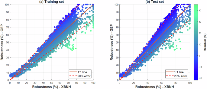
a Training dataset, b test dataset. Colormap shows the variation of residual values per data point. The diagonal solid line (1:1 line) represents the ideal scenario where the predicted values perfectly match the target values. The dashed lines indicate a ± 20% error threshold.
The accuracy of the developed GEP model is quantified in Table 1, detailing various statistical error metrics. The Root Mean Square Error (RMSE) and the Mean Absolute Error (MAE) offer insights into the average magnitude of the errors between the predicted (here the data-driven model) and actual (the dynamic XBNH model) robustness values. RMSE was used to measure the average magnitude of prediction errors, with lower values indicating better accuracy. MAE was employed to capture the average absolute difference between predicted and actual values, providing an interpretable measure of error magnitude. A lower RMSE value in the test set (5.32%) compared to the training set (6.82%) indicates a strong generalization capability of the GEP model. Conversely, the MAE is higher in the test set (6.77%) than in the training set (5.39%), which could imply that while the model predicts most of the data accurately, there are a few outliers with substantial errors that affect the average error magnitude. The Pearson Correlation Coefficient (PCC, also referred to as R-value) is a measure of the linear correlation between the predicted and actual values, with a value range between -1 and 1. Here, the PCC values are high for both datasets (0.94 for training and 0.93 for test), reflecting a strong positive linear relationship. The Coefficient of Determination (R²) quantifies the proportion of the variance in the dependent variable that is predictable from the independent variables. With R² values of 0.88 for the training set and 0.86 for the test set, the model accounts for a substantial portion of the variance.
Optimized vegetation-seawall solutions
The application of the NSGA-II optimization algorithm has successfully navigated the complex landscape of multi-objective optimization for the hybrid vegetation-seawall system, focusing on maximizing robustness and serviceability while minimizing cost. Visualized through the Pareto fronts in Fig. 3, the results elucidate the trade-offs between these competing objectives under varying wave scenarios. The figure, with its panel (a) for robustness, and (b) for serviceability, demonstrates the effectiveness of the NSGA-II in identifying a spectrum of optimal solutions that span across different levels of robustness and serviceability, providing a comprehensive view of how each objective interacts with the cost of implementing the vegetation-seawall system. The robustness analysis reveals a clear, cohesive Pareto front that showcases the algorithm’s ability to delineate solutions that optimize the balance between robustness and cost. Notably, single solutions (per desired robustness) within this Pareto front achieve the highest robustness at the lowest possible cost for robustness levels up to 70%. This finding is pivotal for coastal defense planning, indicating that a universally optimal design may be identified for scenarios up to a certain threshold of wave power. Beyond this threshold, the figure hints at the necessity for tailored designs that are specifically optimized for the prevailing wave conditions at a given location. Such designs diverge from the singular optimal solution, reflecting the algorithm’s sensitivity to varying wave scenarios and its capability to customize design variables (Hsw, Av, and Nv) to achieve higher robustness levels.
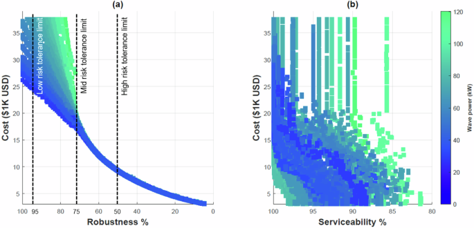
a Robustness. b Serviceability. The colorbar shows the effect of wave power variations on the objectives. Dashed lines on (a) show examples of risk tolerance in terms of the minimum desired robustness.
By considering the specific requirements and constraints associated with different types of coastal infrastructure and communities, the optimized design solutions can be tailored to meet the needs of decision-makers with low, medium, and high-risk tolerance28. By definition, risk tolerance is a measure of the level of risk an organization is willing to accept, expressed in either qualitative or quantitative terms and used as a key criterion when making risk-based decisions29,30. In our context, for example, decision-makers with a low-risk tolerance may focus on solutions that achieve robustness above 95%, ensuring the highest level of protection for critical infrastructure, such as hospitals, power plants, and emergency response facilities. Such areas typically have a low-risk tolerance and require highly robust and reliable coastal protection measures31. Similarly, those with medium (areas with a mix of residential, commercial, and recreational infrastructure) and high-risk tolerance (areas with lower concentrations of critical infrastructure and higher ecological or recreational value) may consider solutions with robustness levels. For example, above 75% and 50%, respectively, balancing coastal protection with other objectives such as cost-effectiveness and ecological benefits. These sample limits are shown in the panel (a) of Fig. 3. By considering these different risk tolerance levels, the optimized design of hybrid vegetation-seawall systems can be adapted to provide targeted solutions for various coastal contexts.
The serviceability analysis, while still yielding acceptable ranges of serviceability (80–100%), does not present as definitive a Pareto front as the robustness analysis. This suggests that the adopted manual search and averaging technique for quantifying the serviceability metric, which was described in the Methods section, may not fully capture the complex, non-linear relationships between the design variables and serviceability. Despite this, the algorithm successfully identifies a range of design solutions that maintain serviceability within the acceptable range, when even considering the worst-case scenario (averaged serviceability in the highest wave power case is 80–85%).
Overall, the algorithm’s performance underscores the importance of scenario-specific optimization, suggesting that while a single, cost-effective design may be feasible for moderate wave conditions, more extreme scenarios necessitate a tailored approach. Moreover, the observed limitations in serviceability optimization highlight areas for future research, particularly the development of more sophisticated models (e.g., neural networks) that can accurately predict serviceability based on design variables. Such advancements could further refine the optimization process, enabling more precise and effective coastal defense strategies.
Risk-Informed desing optimization
RID integrates decision-makers’ risk tolerance into engineering processes, serves as crucial input for the risk management process32. It provides a systematic approach to evaluate trade-offs between performance, cost/damages, and environmental benefits of engineered solutions33. This methodology has evolved as a key component in civil infrastructure planning, particularly within reports and guidelines prepared by the U.S. Army Corps of Engineers (USACE), which emphasizes risk-informed frameworks in the design and evaluation of flood protection systems34,35. Rooted in the USACE’s six-step planning process, risk-informed frameworks blend risk and decision analysis techniques to enhance planning under uncertainty. They allow for transparent comparisons of design alternatives by integrating probabilistic assessments, performance metrics, and stakeholder preferences34,35. By prioritizing multi-criteria decision analysis and stakeholder engagement, risk-informed frameworks enable decision-makers to choose from optimal designs that perform well from an engineering perspective while addressing varying degrees of risk tolerance. This study builds on these principles by proposing a hybrid coastal defense framework that combines natural and engineered features to enhance resilience in flood-prone coastal zones.
In this study, we employed a RID approach by evaluating and selecting among optimized alternative design scenarios that align with different decision-makers’ risk tolerance levels. Real-world examples of sites with different risk tolerance are power plants and evacuation highways for a low risk, commercial districts for a medium risk, and recreational and uninhabited coasts for a high-risk tolerance. This method ensures that the proposed hybrid coastal defense solutions balance robustness, cost-effectiveness, and ecological benefits based on stakeholder-specific priorities. The bi-variate histograms of optimized design variables across different risk tolerance scenarios, as depicted in Fig. 4, reveal intriguing insights into the interplay between seawall height (Hsw), vegetation density (Nsv), and vegetated area (Av) in achieving optimal model resilience-based performance metrics. Here, we consider varying levels of risk tolerance to align the proposed designs with the specific needs and priorities of different stakeholders. Risk tolerance levels have been well studied in civil and infrastructure engineering, with literature providing examples of acceptable risk thresholds across various domains. For instance, NASA’s risk matrix categorizes a “Moderate” likelihood of not meeting performance requirements as 15% to 25%, and “High” likelihood as 25% to 50%, and “Low” likelihood as 2% to 15%, reflecting the tailored use of risk probabilities for decision-making in complex projects36. Similarly, slope stability designs often allow probabilities of failure between 25% and 50% for benches and inter-ramp slopes, reflecting medium to high-risk tolerance levels in civil engineering projects37. Drawing from these suggestions, we adopted three levels of risk tolerance in our framework: low (5% failure chance, 95% robustness), medium (25% failure chance, 75% robustness), and high (50% failure chance, 50% robustness).
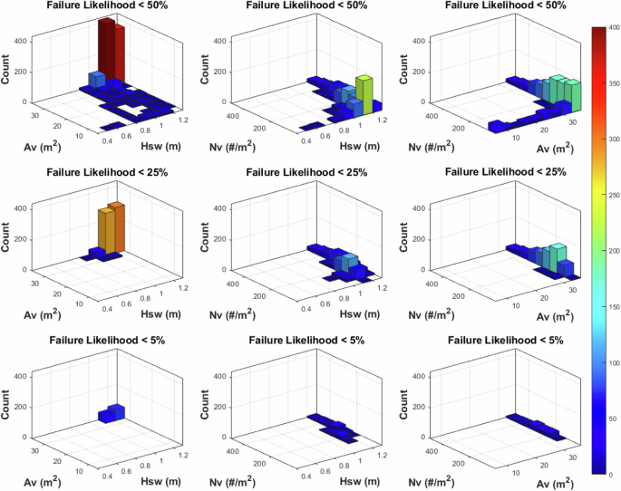
Optimized solutions are illustrated for low (bottom row), medium (mid row), and high (upper row) risk tolerance based on the expected robustness of the system and failure (overtopping) likelihood. Colorbar shows the frequency of solutions.
For a high-risk tolerance (where there is a 50% chance of overtopping, i.e., system failure), the results in the first row of Fig. 4 show that the majority of optimized values, situated on the Pareto front in Fig. 3, occur when the seawall height Hsw surpasses 0.8 m, the vegetation density Nv falls below 100 stems.m–2, and the vegetated area Av exceeds 30 m2. This finding suggests that increasing vegetation density (beyond 100 stems.m–2) within the same area does not significantly enhance the model’s performance metrics. Instead, a more effective approach involves expanding the vegetated area while maintaining a density below 100 stems.m-2. Furthermore, Fig. 4 highlights the importance of maintaining a minimum seawall height of 0.8 m (~75% of the Base Flood Elevation) to ensure sufficient capacity for accommodating extreme wave run-ups that cannot be effectively mitigated by coastal vegetation alone. Increasing vegetation density beyond 100 stems.m-2 would incur additional project costs without yielding substantial improvements in system resiliency metrics in high-risk tolerable areas. Alternatively, allocating resources towards expanding the vegetated area proves to be a more effective strategy, as it promotes wave energy dissipation further from the shore, ultimately reducing the wave impact on the hybrid structure. The general trend of available solutions in Fig. 4 indicates that as the risk tolerance of decision-makers decreases (e.g., for critical coastal infrastructure), designs tend to lean more heavily towards gray structures (seawalls) for enhanced robustness in front of extreme wave scenarios.
In contrast, the optimized solutions for high robustness scenarios (less than 5% risk of system failure) are primarily associated with moderate vegetation density values (Nv~250) within the feasible range of Nv. This finding indicates that investing in expanding the vegetation area may take precedence over increasing vegetation density for stakeholders with a low-risk tolerance when allocating project costs. However, it is important to note that vegetation density could play a crucial role in designs that aim to guarantee the lowest possible flood risk. In such cases, adequate vegetation area and density are essential to ensure maximum protection against flood hazards. Therefore, we can also conclude that in cases where expanding the vegetated area in the intertidal zone is not feasible, or may not guarantee the robustness needed for flood mitigation purposes, optimized results can still be achieved by increasing vegetation density. This approach allows effectively utilizing available space while maximizing the system’s resiliency. These findings underscore the delicate balance between seawall height, vegetation density, and vegetation area in optimizing the performance of hybrid coastal protection structures. By carefully considering these design variables and their interactions, coastal engineers and managers can develop more resilient and cost-effective solutions to mitigate the impacts of extreme wave events on coastal communities and infrastructure.
Discussion
The results of this study provide insights into the performance and optimization of hybrid vegetation-seawall systems for coastal protection against extreme wave conditions. The XBNH model simulations dataset analysis has revealed the relative importance of design variables (seawall height, vegetation area, and vegetation density) in influencing the system’s performance metrics, including wave runup, overtopping volume, robustness, and flood serviceability. The sensitivity analysis showed that increasing seawall height has a more pronounced effect on limiting overtopping volume and enhancing robustness, consistent with the conventional role of seawalls as primary physical barriers against extreme waves. However, the analysis also highlights the critical contribution of vegetation in reducing wave runup, particularly when vegetation density and area exceed a certain threshold. This finding emphasizes that vegetation below a minimum density or area may have negligible effects on system performance. Therefore, maintaining a balanced vegetation density and area is essential to harness the fundamental benefits of NBSs, reinforcing the importance of integrating these elements with engineered structures for effective and sustainable coastal protection.
The resilience-based metrics, i.e., robustness and flood serviceability, have exhibited different sensitivities to the design variables. While the system robustness is moderately sensitive to the seawall height, the vegetation characteristics substantially impact both robustness and flood serviceability. This finding suggests that the strategic incorporation of vegetation into coastal defense systems can significantly contribute to their overall resilience, as the ability of vegetation to absorb and dissipate wave energy, thereby reducing the wave runup on the system. Moreover, the results indicate that beyond a certain vegetation area, overtopping can be effectively mitigated in all cases of seawall height tested here, suggesting that prioritizing the optimization of vegetation characteristics can lead to more cost-effective and sustainable coastal protection strategies. Given the constraints on the maximum seawall height and the wider range for vegetation area and density in our case study, the cost analysis has also revealed that the total cost of the hybrid system could be more influenced by the vegetation characteristics than the seawall height in this case.
The GEP model has demonstrated a high accuracy in predicting the system’s robustness based on the input variables, with strong correlations between the predicted and target values in both the training and test datasets. This result underlines the potential of data-driven techniques, in developing efficient and reliable models for coastal engineering applications. The ability to accurately predict the performance of coastal defense systems based on key design variables can greatly facilitate the optimization process and support informed decision-making. The success of the GEP model can be attributed to its capability to evolve complex mathematical expressions that capture the non-linear relationships between the input variables and the system’s performance, without requiring a priori assumptions about the model structure.
Further in the utilized optimization framework, the results suggest that a set of optimal design solutions (in Pareto fronts) can be identified that maximizes robustness at the lowest possible cost over a range of lower wave powers tested here. However, for higher robustness levels and more extreme wave conditions, the optimization results underscore the need for site-specific designs that are tailored to the environmental conditions, highlighting the importance of considering the local context, including the wave climate, bathymetry, and ecosystem characteristics, when designing coastal defense systems. The optimization results also reveal that expanding the vegetated area while maintaining a moderate vegetation density is more effective in enhancing the system’s resilience compared to increasing the vegetation density within a limited area. This finding also offers insights for coastal restoration and management strategies, as it suggests that prioritizing the spatial extent of vegetation, rather than solely focusing on increasing density, can lead to more effective coastal protection. The results further highlight the importance of maintaining a minimum seawall height to ensure sufficient capacity for accommodating extreme wave runups that cannot be effectively mitigated by vegetation alone. This insight emphasizes the complementary roles of engineered and nature-based components in hybrid coastal defense systems and the need for a balanced approach that considers both structural integrity and ecological enhancement. The necessity of a minimum seawall height can be attributed to the limitations of vegetation in attenuating extremely high waves and the importance of providing a last line of defense to prevent overtopping and flooding during severe events.
It is essential to acknowledge the limitations of this study and the aspects that have not been extensively discussed. The potential damage to vegetation during extreme events and its impact on the long-term performance of the hybrid system warrants further investigation, as this could affect the system’s robustness, resourcefulness, recovery, and rapidity during and after an extreme event. Additionally, the study does not explicitly address the effects of beach erosion, which are important considerations in the overall resilience of coastal systems. Future research could expand the optimization framework to incorporate these factors, examining the beach’s robustness, resourcefulness, recovery, and rapidity during and after extreme events, to provide a more comprehensive understanding of the system’s resilience.
The reliability of the proposed framework is rooted in its ability to incorporate RID principles and its validation under real-world conditions. Long-term monitoring of existing hybrid systems in varied coastal environments would enable the evaluation of their performance under different wave climates, storm events, and risk levels. These studies could also capture dynamic factors such as vegetation growth, seasonal changes, and damage during extreme events, providing insights into the long-term resilience of these systems under uncertainty. Integrating such empirical evidence into the optimization framework would enhance its robustness and its ability to support decision-makers in selecting designs aligned with specific risk tolerance levels.
While the proposed optimization framework demonstrates significant potential for advancing hybrid coastal defense designs, its practical implementation involves several challenges inherent to a risk-informed approach. Accurate modeling requires high-resolution data on wave dynamics, vegetation characteristics, and site-specific conditions—data that may be scarce in regions with limited monitoring infrastructure. Finally, although guidelines for designing nature-based features have emerged since last decade, such as the guideline of Use of Natural and Nature-based Features for Coastal Resilience38 and International Guidelines On Natural And Nature-Based Features For Flood Risk Management39, there is a gap in the optimum design guidelines specifically tailored for hybrid engineering and nature-based structures for flood mitigation. Therefore, the main contribution of the present study is dedicated to providing design insights for these systems. The optimization framework presented in this study can also be expanded to other hybrid green-gray flood mitigation systems beyond the vegetation-seawall systems.
Methods
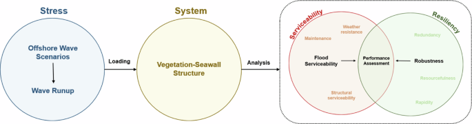
The framework components are depicted in Fig. 5, and described below. components are shown in Fig. 1
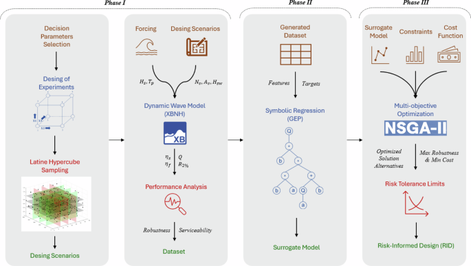
The sampling, design scenarios, hydrodynamic modeling, and resilience analysis are carried out in Phase I. In Phase II, generated dataset in Phase I is utilized to train a surrogate model as an objective function in the multi-objective optimization process. In Phase III, the surrogate model and the cost function are used to find the optimal balance of the system design parameters, and the suggested designs are offered based on risk tolerance limits.
Dynamic wave model
The open-source XBeach non-hydrostatic (XBNH) model, developed by ref. 40, is employed in this study to simulate wave runup and overtopping over a seawall fronted by a vegetated beach, and consequently to generate the performance metric dataset for the training of the data-driven model mentioned earlier. XBNH is a phase-resolving wave model that solves the depth-averaged non-linear shallow water equations coupled with a non-hydrostatic pressure correction term. The accuracy of the model relies on the calibration of several input variables, including the maxbrsteep, which sets a limit for the rate of change in surface elevation at wave breaking points, as identified by ref. 41. The horizontal viscosity in XBNH is determined by multiplying the Smagorinsky-based viscosity by a user-defined constant, breakviscfac, which ranges from 1 to 3. Based on the sensitivity analysis conducted by ref. 42, which utilized several laboratory and field datasets, we selected maxbrsteep as 0.65 and breakviscfac as 1.5 to ensure model accuracy across various case studies. The one-dimensional governing equations in XBNH are:
where (x) and (t) signify the spatial and temporal coordinates, respectively, (eta) denotes the elevation of the water surface, (u) represents the depth-averaged velocity, n is the Manning’s roughness coefficient, g is the gravitational acceleration, and (d) indicates the local water depth. The horizontal viscosity is depicted by ({nu }_{h}), the term (bar{q}) refers to the depth-averaged dynamic pressure, and ({tau }_{beta ,x}) corresponds to the bed shear stress as per43. The model considers vegetation effects through a vegetation force determined as per44, where ({F}_{v}) is the force applied by the vegetation to the mean flow over the vegetation’s height45,46,47:
In this equation, CD is the bulk vegetation drag coefficient, bv is the stem diameter, and Nv is the vegetation density. The drag coefficient in XBNH is a calibration constant, which can alternatively be estimated using an empirical formula based on flow and vegetation characteristics, as suggested by ref. 48. This study employs the empirical formula from ref. 49, which has been effectively integrated into various hydrodynamic and wave models10,50,51.
Here ({R}_{p}) represents the plant Reynolds number, which is calculated as (u{b}_{v}/nu) where (u) is the acting flow velocity on the submerged vegetation50. Both ({alpha }_{0}) and ({alpha }_{1}) are empirical coefficients influenced by the volumetric fraction of the vegetation, denoted as (varphi), taken from50.
Study area, wave scenarios, and vegetation properties
We implement our methodology to a beach profile site in Longport, New Jersey, United States, labeled as Profile #126 in the New Jersey Beach Profile Network52. Positioned at the southern end of Absecon Island, along 17th Street in Longport (refer to Fig. 6), this location features a narrow, low-elevation beach adjacent to a concrete seawall. Historical weather events have underscored the vulnerability of this beach-seawall system to extreme sea levels, as exemplified during Hurricane Sandy in 2012 when storm-induced waves overtopped the seawall, leading to extensive flooding and considerable damage to adjacent residential areas. We develop a computational domain for the study site using elevation data from historical measurements during 1989–2011. The measurements are collected by the Coastal Research Center (CRC) at Stockton University52.
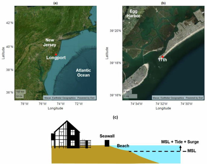
a Arial view; b local perspective; and c profile schematic of the site with an added hypothetical intertidal vegetation zone. Hsw is the seawall height, and Av and Nv are the vegetation area and density, respectively.
In our analysis of the seawall’s robustness and serviceability, we aim to explore the influence of optimized vegetation and seawall features on the system response to different extreme wave scenarios. The wave scenarios utilized in this investigation derive from a synthetic hurricane dataset from53, who explored the effects of climate change on wind-generated waves from major hurricanes impacting New Jersey’s coast. In total, we consider 50 wave scenarios. Figure 7 illustrates the range of wave power, significant wave heights (HS), and peak wave periods (TP) simulated for this study. We consider waves with TP values ranging from 4 to 14.7 s and HS values reaching up to 4.6 m. These wave parameters are employed to generate water level time series at the XBeach model’s offshore boundary using a Joint North Sea Wave Project (JONSWAP) spectrum. The model’s offshore boundary is established at a water depth of ~15 m. Each wave scenario undergoes a 15-min simulation, producing time series data for wave runup and overtopping. From these time series, the two percent exceedance wave runup R2% (which is a standard metric in coastal engineering), and overtopping volume are calculated.
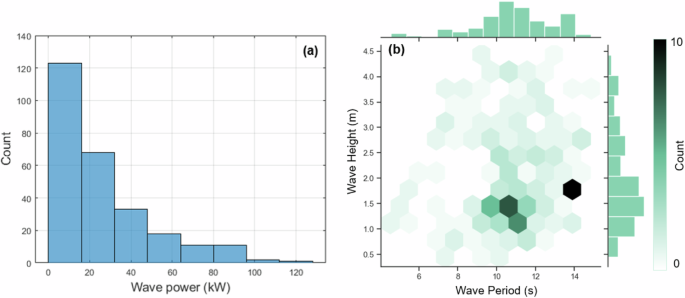
a Wave power, b scatters and distribution of wave height and wave period.
In our optimization algorithm, the maximum height of the seawall (Hsw) is a constraint and thus needs to be predefined. Here it is determined based on the base flood elevation (BFE) – associated with 100-year flood – selected from the US Federal Emergency Management Agency (FEMA) flood maps54. The BFE at our study site is 9 ft (2.78 m) relative to the National Geodetic Vertical Datum of 1929 (NGVD 29), and 10.8 ft (3.29 m) relative to mean sea level (MSL). Given that the beach elevation at the toe of the seawall is 2 m above MSL, we set the maximum seawall height (vertical distance from the toe to the crest) to 1.29 m. Given that residential areas are typically designed to withstand a 100-year storm, constructing walls higher than this standard elevation may not significantly enhance the structure’s resilience during its lifetime. Moreover, such a design choice could lead to undesirable socioeconomic impacts on the community (e.g., an obstructed ocean view). These may include obstructing views from buildings and limiting recreational spaces, among other potential consequences. Furthermore, the increased construction cost associated with very high seawalls may not yield a commensurate increase in mitigative effect (beyond a certain extent).
For the vegetation type, we adopt Saltmarsh Cordgrass (Spartina alterniflora), which is a perennial grass found along the Atlantic Coast, ranging in height from 0.1 to over 2 m55. This native, warm-season grass forms dense colonies in coastal wetlands and is highly tolerant to fluctuating water depths and salinity. The plant’s height varies according to site conditions, with flat leaf blades typically 0.3 to 0.5 m long, tapering to a long inward-rolled tip55. Since this plant thrives within the tidal range, the maximum length of the vegetation zone at our study site can range from zero to 36 m, the length of the beach within the intertidal zone. Stem density is quite variable but usually averages about 100–200 stems per square meter (10–20 stems per square foot) and can range as high as 500 stems per square meter56. As an example from a living shoreline project at a nearby site, the density of spartina alterniflora in the Gardener’s basin living shoreline project57 is roughly 100 stems per square meter. Based on the characteristics of spartina alterniflora discussed above, the design variable ranges in our optimization problem are set to those shown in Table 2.
To test our methodology under extreme events, we set the initial water surface elevation to 2 m above MSL. This water level resembles storm tides at the study site during extreme events. For example, according to measurements at the NOAA tide gauge at Atlantic City, which is located near our study site, the peak water level during Hurricane Sandy in 2012 was 2 m above MSL.
Performance metrics: definitions and measures
The concept of coastal resilience pertains to the capacity of coastal protection mechanisms to resist and recover from disturbances such as storm surges, waves, and other coastal hazards58,59. As this research emphasizes the structural response to storm incidents over short periods, it is crucial to define the systems and stresses when discussing the resilience components.
Considered as the system in this study, the vegetation-seawall system provides a physical barrier against storm tides and high wave events. These events usually make wave runup, which is a critical stressor for the vegetation-seawall system, describing the wave-induced uprush of water above still water level reaching the seawall60. It is a key factor in designing coastal protection measures as it directly impacts the wave overtopping rates and the potential for flooding. The extent of wave runup is influenced by several factors including storm intensity, sea level rise, beach slope, and the presence of coastal vegetation61.
Resilience comprises four key components: robustness, resourcefulness, redundancy, and rapidity62. While these components are crucial for assessing the resilience of systems under various stressors, in the context of evaluating the capacity of a vegetation-seawall system to remain robust during extreme events, the emphasis on recovery, resourcefulness, and rapidity may not be as relevant. This is particularly true when the recovery is primarily due to a decrease in stress rather than the system’s inherent recovery mechanisms. Therefore, in scenarios where the focus is on the system’s ability to maintain robustness in a very short time during extreme events, considerations of recovery, resourcefulness, and rapidity may not align with the immediate demands of the situation, which is the case in this study. Instead, prioritizing robustness and the system’s inherent ability to withstand stress in real time becomes paramount for effective resilience in such contexts. To assess the vegetation-seawall system performance, we build upon the foundational work established in ref. 15, where they developed novel metrics for assessing the robustness and flood serviceability of hybrid coastal defense systems consisting of beaches and seawalls. We adopt and apply the established metrics of robustness and flood serviceability to a hybrid vegetation-seawall structure, as illustrated in Fig. 8
Definitions of the system, stress, and the selected resiliency metrics to carry out performance analysis of the hybrid vegetation-seawall coastal system.
Metric I: Robustness
From the perspective of civil infrastructure resiliency, robustness is defined by the system’s ability to absorb stress (or disturbance) and maintain its functionality under various conditions, highlighting its capacity to handle unexpected stresses without substantial degradation or loss of functionality58,63. In coastal engineering, robustness is generally defined as the capacity of a coastal defense system to withstand extreme conditions without failure, focusing on its ability to resist significant damage from events like storm surges and high waves under uncertainty64,65. Following these definitions in this methodology, robustness represents the capability of the vegetation-seawall system to sustain its operational integrity and efficacy amid extreme wave scenarios. Given the study’s prioritization of wave runup as the principal stress factor affecting the hybrid beach-seawall system, maintaining system robustness is crucial for the successful mitigation of wave runup and the prevention of seawall overtopping. A vegetation-seawall system’s peak performance is achieved when wave runup is fully contained by the intertidal vegetation component, preventing any runup impact on the seawall (as illustrated in Fig. 9). In contrast, the system fails to perform its intended function when the wave runup reaches the crest of the seawall, resulting in wave overtopping. Therefore, the seawall’s dry height becomes a critical measure of the system’s performance.
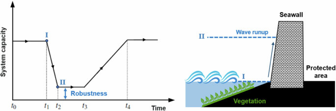
Simplified diagram of systems performance curve (on the left), and associated states when wave runup stressing the vegetation-seawall system (on the right). The desirable performance of the structure before the disturbance (stress) happens at state (I), and system capacity decreases as runup stresses the system to a certain extent during the storm (state II).
Amini et al.25 developed a metric to quantify the robustness of a seawall by measuring the available dry height on the seawall, which indicates its capacity to withstand wave runup without leading to overtopping. This metric is based on a robustness score (RS) for each storm event, representing the integral of the time series of seawall dry height over the duration of the storm as formulated below. This score provides a quantitative measure of the system’s ability to maintain functionality under stress conditions, with a higher RS indicating greater robustness.
where t1 and t2 indicate the beginning and end of a storm event, and t signifies the time step. The robustness metric can then be quantified by time averaging the robustness score (over the storm duration) and being normalized using the seawall height.
where T is the total duration of the storm.
Metric II: flood serviceability
The general definition of structure serviceability is the ability of a structure to continue operating under normal and extreme conditions, maintaining its intended function without requiring excessive maintenance or repair66. Serviceability can also be defined as the ratio of satisfied demand after the stress or shock to the estimated total demand at the highest stress or shock15. In the context of the coastal vegetation-seawall system here, when the flood level behind the seawall surpasses a predefined threshold, such as the BFE which is a basis for structural reliability measurements and flood insurance coverage, we consider the system loses its flood serviceability (referred to as “serviceability” hereafter) as it can no longer provide the intended flood protection. Inspired by the post-flood damage assessment practices, which involve evaluating High Water Mark surveys, we quantify the flood serviceability based on the maximum water level behind the seawall during a storm event and compare it with the BFE from the United States Federal Emergency Management Agency (FEMA). Despite the loss of robustness during the overtopping, the seawall continues to offer service by mitigating the flood depth in the area behind it. This may result in minor flooding, compared to the potential significant flood when there is no seawall in place. As an example, shown in Fig. 10, the immediate flooding once the seawall is overtopped impacts the area behind the seawall; nevertheless, the seawall managed to control it to be lower than BFE (state I, serviceability < 100%). As the storm continues, the flood depth behind the seawall increases and finally reaches the BFE level. At this flood level, the seawall experiences a state of total failure (state II) and will no longer mitigate the incoming flood (serviceability = 0%).
States of the flood depth behind the seawall, on the left, and the increase of flood elevation to reach the flood serviceability reference in this study (i.e., BFE), on the right.
We use the flood serviceability metric introduced by Amini et al.50 to quantify the vegetation-seawall system’s effectiveness in controlling flood depth behind the seawall during overtopping events. This metric is defined as the minimum ratio of the flood capacity behind the seawall to a predetermined BFE. It reflects the degree to which the system can continue to provide service by mitigating flooding, even when robustness is compromised.
where (0le ile Delta T) signifies the time steps during the overtopping of the seawall (∆T is the total duration that overtopping occurs during a storm). A “total failure” takes place when the flood depth exceeds BFE.
The robustness and serviceability metrics described above are illustrated using a conceptual model in Fig. 11. After applying stress (wave runup) on the system, the system’s robustness starts reducing from its maximum value of 100% (Phase 1). The robustness reduces to zero when the wave runup reaches the crest of the seawall and overtopping initiates (Phase 2). From this moment on, the area behind the seawall is flooded, even though the seawall is still serving its function by retaining the flood depth below BFE (Phase 3) until total failure occurs (Phase 4).
Phase 1 denotes no system failure. Phase 2 shows maintained flood serviceability but a zero-robustness state. Phase 3 indicates zero robustness with decreasing flood serviceability. Phase 4 marks total failure state when the flood level behind the seawall reaches or exceeds the BFE.
Cost analysis
Minimizing the cost of the vegetation-seawall system is one of the two objective functions in the optimization problem. Here, we developed a cost formula based on the previously reported costs associated with different shoreline stabilization projects, using a methodology outlined in ref. 67 and data from 16 projects in Coastal New England, detailed in ref. 68. The focus is on both concrete seawalls and Spartina alterniflora, as a hybrid vegetation-seawall solution. The total cost of a vegetation-seawall system is calculated as the sum of the initial cost (IC), damage cost (DC), maintenance cost (MC), and replacement cost (RC). The IC is the foundational expense for constructing the measure, including factors such as material, labor, and overall bulk expenses. According to69, the IC for living shoreline projects ranged from $88 to $2018 per linear foot, whereas conventional projects ranged from $462 to $3448 per linear foot.
The DC is related to repairs following significant storm events (like hurricanes) under a moderate overtopping and scour scenario. This study uses the storm damage percentage for a 25-year storm as outlined in ref. 69. The Hudson River Sustainable Shorelines Project (HRSSP) framework67 indicates that damage costs can be calculated as a percentage of the IC, with specific adjustments based on the frequency and severity of expected storm events. The RC refers to the expense of completely rebuilding the structure after a certain period, typically due to material degradation. The replacement costs for conventional projects are more concentrated at discrete times, whereas living shorelines may incur smaller, more frequent replacement costs. The MC involves the routine upkeep required for these stabilization means. It is assumed that the coastal vegetation does not need to be fully replaced, and only routine monitoring, maintenance, and partial planting (mentioned as repairs) would be enough during the project’s lifetime. The HRSSP framework, as applied by ref. 69, breaks down maintenance into routine inspections, minor repairs, and adaptive management. For instance, monitoring and adaptive management costs for living shoreline projects can sometimes exceed construction costs due to the need for ongoing ecological assessments and adjustments.
To account for the time value of money and the impact of inflation over the 25-year lifetime of the project, we incorporate appropriate discount and inflation rates in our cost analysis. The discount rate will be based on the most recent guidance provided by the U.S. Army Corps of Engineers (USACE) in their Economic Guidance Memorandum (EGM) 23-01, Federal Interest Rates for Corps of Engineers Projects for Fiscal Year 202370. As per this guidance, we will use a discount rate of 2.5% for our analysis. Additionally, we will use an inflation rate of 3.4% based on the latest available data from the U.S. Bureau of Labor Statistics71 and the Congressional Budget Office’s (CBO) long-term inflation projections72. These rates will be applied consistently throughout the cost analysis to ensure that the estimated costs accurately reflect the expected future value of the project over its 25-year lifetime. To that end, we first calculate the Future Value (FV) of the costs using the inflation rate, as follows:
where PV is the present value (initial cost), i is the inflation rate (3.4%), and n is the number of years into the future the cost is incurred.
The mean costs of each category are presented in Table 3 for seawall and in Table 4 for vegetation projects. These costs provide a bulk estimation per unit length for each gray/green solution. The median costs shown in the tables are used in the present study.
After calculating the inflated costs, these costs are combined using the following equation to approximate the total cost of a hybrid vegetation-seawall solution. We estimate the total cost per unit length using the following formulation that accounts for initial, damage, replacement, maintenance, and repair costs during a 25-year lifetime.
Where TChybrid is the total cost of hybrid vegetation-seawall system, ({{TC}}_{S}) is the total cost of seawall construction per linear meter, and ({{TC}}_{v}) is the total cost of the coastal vegetation project, where there is no seawall in place.
The total cost of a standalone seawall project can be approximated with:
The shape adjustment factor, ({F}_{v}), quantifies the volumetric impact of the seawall face slope. For a vertical (90°) slope, resembling a rectangular shape, ({F}_{v}) equals 1. When the slope adjusts to 45°, creating a trapezoidal shape, the volume increases to 1.5 times that of the rectangular form, setting ({F}_{v}) at 1.5. ({F}_{e}) is the ratio that approximates the benefit of vegetation in terms of its effect on the degradation of the seawall over time. Here it is assumed that the influence of vegetation on seawall damage mitigation is linearly proportional to the area and density of the vegetation, with maximal vegetation coverage and density providing complete damage prevention (according to Table 2), starting from 1 (in the case of maximum Av*Nv), linearly decreased to zero (for the minimum Av*Nv). For the sake of simplification, this relationship is presumed to be linear, diminishing progressively as vegetation coverage decreases.
The total cost of the vegetation construction can be approximated with:
Here ({{N}_{v}}_{{avg}}) is the average vegetation density in the implemented projects in New Jersey (~90 stems per square meter).
Regarding the coastal vegetation benefits, they provide a range of additional ecosystem services that, while not considered in this study, could be integrated into the proposed framework to enhance its comprehensiveness and support their maximization. An example of such services include sediment stabilization and erosion control, which are critical for maintaining shoreline integrity and reducing sediment transport costs73. Vegetation also plays a vital role in nutrient cycling, aiding in the reduction of nitrogen and phosphorus loads in coastal waters, which mitigates eutrophication risks and enhances marine ecosystem health74. Furthermore, the aesthetic and recreational value of vegetated coastal areas supports tourism and increases property values in adjacent communities75,76. Possible incorporation of these co-benefits into the framework through valuation metrics and considering them as another optimization objective in the framework could provide a more holistic assessment of hybrid coastal protection systems, ensuring the alignment of engineering and environmental objectives.
Design of experiments
As discussed earlier, seawall height (Hsw), and vegetation area (Av) and density (Nv) are the design variables in the optimization problem. When conducting numerical experiments to generate the dataset for training the data-driven model, it’s crucial to choose samples that cover a wide range within the possible values to accurately represent the design variables. However, too many samples will make numerical experiments computationally demanding. To tackle this issue, our study adopts methods from the Design of Experiments field, specifically the Full Factorial Experiment Design (FFED). This statistical approach involves experiments with two or more variables (V) or factors, each having different potential intervals or levels (L). The design ensures that every possible combination of these levels across the variable ranges is tested. This allows for a comprehensive examination of how each variable and their interactions affect the outcome. To ensure a thorough representation of all possible values, we divide the feasible range for each design variable into four equal levels (as detailed in Table 5). Our sampling strategy is then designed to cover all these levels extensively. Building on this approach, the number of samples required is determined by ({L}^{V}), where L represents the number of levels and V is the number of variables (factors). In our case, with three variables (V = 3, Hsw, Av, and Nv) and four intervals (L = 4), this calculation results in 43, meaning we need 64 samples (per wave scenario described earlier) to test every possible combination of levels and parameters.
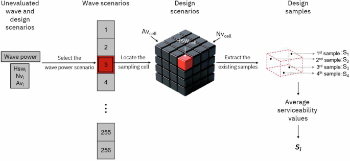
Sampling method
Once the intervals of design variables are determined (Table 4), we sampled combinations of Hsw, Av, and Nv within each interval. This combination of design variables, along with wave scenario parameters, wave height (Hs) and wave period (Tp), are used in the XNBH model to generate the training dataset for the data-driven model. We use Latin Hypercube Sampling (LHS)77 for sampling from cells. Here a cell is a 3D space that contains 4 samples (combination) of design variables, each in a given Interval (as depicted in Fig. 12). LHS is a statistical method that generates random samples of parameter values from a multidimensional distribution. The method operates by dividing the range of each parameter into intervals of equal probability and then randomly sampling points from each interval, ensuring that each sample is representative of the entire parameter space. LHS was chosen for its effectiveness in generating evenly distributed random samples across the entire range of each variable. For each cell, four samples were generated, resulting in 256 (64 cells x 4 samples) distinct data points. This structured approach ensured that each segment of the parameter space was equally represented, maintaining the integrity of the sampling methodology. To visualize the sampled datapoints in our methodology, we focus primarily on 2D projections to elucidate the pairwise scatter of the variables. In Fig. 12, each panel (b-d) shows two variables (e.g., Nv and Hsw in panel b) and color coding is utilized to distinguish intervals of the third variable. The range of the third variable was segmented into four intervals, each denoted by a distinct color (blue, green, red, and gold). Interval boundaries were marked in the 2D projections for enhanced clarity. Given the limitations of 2D projections of the samples (Fig. 12b–d), 16 samples are shown in 2D bi-variate projections, however, each four of them belong to a certain class of the third variable (shown in the legends), distinguished by their colors. This way, only 4 samples are taken from each cubic sample cell in a 3D search space (Fig. 12a).
Each interval represents a range of values for design variables: seawall height (Hsw), vegetation area (Av), and vegetation density (Nv). Sampling points within each interval are indicated, with points distributed using Latin Hypercube Sampling (LHS) to ensure even representation across the design space. a 3D sampling area, b 2D bi-variate projection for seawall height over vegetation density, c 2D bi-variate projection for seawall height over vegetation area, d 2D bi-variate projection for vegetation density over vegetation area. Dashed lines show interval boundaries based on the Design of Experiments method.
Data-driven symbolic regression model for the robustness metric
To discover the non-linear mathematical representation that most accurately describes the relationship between input variables (wave power, seawall height, and vegetation characteristics) and output response (system robustness), we employed GEP as a data-driven symbolic regression model. The general form of the mathematical representation is:
This evolutionary algorithm is adopted for generating models or solutions by emulating natural evolutionary processes such as selection, mutation, and recombination. Developed by ref. 78, GEP transcends its predecessors—Genetic Algorithms (GA) and Genetic Programming (GP)—by integrating the robustness of genetic algorithms with the expressive power of genetic programming into a singular, cohesive framework79. The framework adopted here represents solutions as linear strings of characters, like chromosomes in DNA, which are subsequently expressed as tree structures for evaluation. This hallmark feature facilitates a blend of genetic algorithms’ simplicity and efficiency with the flexibility and depth of genetic programming80. Compared to conventional approaches, the inclusion of a GEP-based regression model in this study provides an innovative solution to the computational inefficiencies of iterative dynamic wave simulations. This enables efficient exploration of a large design space with low computational cost, which is critical for optimizing hybrid solutions under varying environmental conditions.
As illustrated in Fig. 13, GEP initiates with the generation of chromosomes population and genes. Given the complex interrelation of features-targets, we train the model with 64 chromosomes each having 3 genes, which can encode different parts of the solution. The model then generates linear strings comprised of symbols representing functions (e.g., mathematical operations) and terminals (variables or constants). These elements are selected from a pre-defined set pertinent to the problem81. Selected mathematical operations used in our model generation are listed in Table 6, after preliminary trial and error. Each chromosome is structured into a head, housing symbols for both functions and terminals (head size = 4 in our experiments), and a tail, composed solely of terminals. The tail’s length, dictated by the head’s length and the maximum arity of the functions employed, ensures every tree structure expressed by the chromosome is syntactically valid. The evolutionary journey begins as these chromosomes undergo translation into their corresponding expression trees, which are evaluated to measure their fitness relative to the problem at hand82. Fitness is a measure of a chromosome’s efficacy in problem-solving or its alignment with the training data. The fittest chromosomes are earmarked for reproduction, passing their genetic material to subsequent generations through mechanisms like mutation, recombination (or crossover), and transposition, thereby introducing genetic diversity and enabling solution space exploration.
Workflow of the Gene Expression Programming, including program preparation, execution, and selection (yellow boxes), genetic replication or mutation (blue boxes), transposition (green boxes), and recombination (red boxes)78.
In our study, we employed the Quartile Root Relative Squared Error (Quartile RRSE) as the fitness function to evaluate the performance of our model. The Quartile RRSE is calculated using the following formula where ft (k) represents the actual (true) values, fe (k) the predicted values by the model, and (overline{{f}_{t}left(kright)}) the median of the actual values, focusing the calculation on the central portion of the data distribution. Finally, ({N}_{s}) is the total number of data points.
This approach is designed to minimize the influence of outliers, making the fitness evaluation more robust and ensuring that the models evolved by our GEP framework are not only accurate but also resilient against extreme data values. The adoption of Quartile RRSE aligns with our goal of crafting models that consistently deliver reliable performance across diverse scenarios, offering a judicious balance between accuracy and robustness in predictive modeling.
The evolutionary dynamism enables GEP with the capacity to evolve complex, multidimensional models that elucidate the intrinsic patterns or relationships within XBNH-generated data without necessitating a pre-defined model structure. This attribute makes GEP particularly effective in symbolic regression endeavors, where the objective is to unearth mathematical expressions that succinctly encapsulate the relationship between input variables and outputs based on the numerical dataset we have here. The generated surrogate model polynomial is detailed in the Supplementary Information section in the form of expression trees.
To ensure the robustness and generalizability of the GEP model, the dataset generated by the XBeach non-hydrostatic model (XBNH) was randomly divided into training and testing subsets. Specifically, 70% (=8960 rows) of the data was allocated for training, allowing the GEP model to learn the relationships between input variables and performance metrics, while the remaining 30% (=3840 rows) was reserved for testing to evaluate the model’s predictive capability on unseen data. This division strategy ensures that both subsets are representative of the full range of design variables (seawall height, vegetation area, vegetation density) and storm wave scenarios. Random sampling was used to minimize bias and avoid overfitting. Optimal values for hyper parameters are selected following the values suggested by a similar work that used GEP to predict wave runup on beaches83. Through GEP’s evolutionary algorithm, we aimed to identify models that not only predict the hybrid system’s robustness metric with high accuracy but also offer insights into the interplay between these critical design factors.
Quantifying serviceability metric
A similar GEP model has been developed for the serviceability metric. However, we found the GEP model struggles to formulate an accurate predictive expression, which can be due to the highly non-linear and complex relation between this metric and its influencing factors (wave power, Hsw, Av, and Nv). Consequently, we adopt a search with averaging approximation technique for calculating the serviceability metric in the optimization algorithm. Using this method, for any specific set of input design variables, we initially identify the associated 3D search space for that particular wave scenario. We then traverse this 3D space across all 64 sampling cells to ascertain the cell in which the given inputs are located. Subsequently, we calculate the average of the values from the four samples within that cell (for which we already have the serviceability values from XNBH runs) and apply this average as the estimated serviceability for the given point. While this approach may not guarantee the highest precision, it nonetheless provides satisfactory outcomes.
Where i is the evaluation number, N = 4, and ({{bf{x}}}_{{cell}}) is the vector of values of all design variables within the closest cell where the given point is located. The process is illustrated in Fig. 14.
Serviceability approximation procedure for unevaluated design scenarios.
Multi-objective optimization
In this subsection, we present the application of the Non-dominated Sorting Genetic Algorithm II (NSGA-II)84 in our problem to maximize robustness and serviceability and minimize the cost for hybrid vegetation-seawall systems. NSGA-II is an evolutionary algorithm that is particularly well-suited for solving multi-modal problems with multiple conflicting objectives. It is an extension of the genetic algorithm (GA) framework, incorporating mechanisms to preserve diversity and emphasize non-dominated solutions85,86. The algorithm begins with an initial population of solutions, each encoded as a chromosome. The fitness of each solution is evaluated based on the objectives, which in this case are the maximization of robustness and serviceability and the minimization of cost, as defined by the cost function detailed in the cost analysis section. Here, we aim to solve the following optimization problem:
where:
Subject to constraints:
The optimization constraints were derived based on the ranges and parameters detailed in the subsection “Design of experiments” of section “Methods” (Section 4.5, Table 5) and Study Site Characteristics (Section 4.2, Table 2). The NSGA-II algorithm utilized here starts with a non-dominated sorting process. The combined parent and offspring population is sorted into different fronts based on non-domination levels85. A solution (x) is said to dominate (y) if it is no worse than (y) in all objectives and better in at least one objective. Mathematically, this can be expressed as:
Where ({f}_{k}) represents the ith objective function. The search procedure of the algorithm and a sudo code is presented in the Supplementary Information.
The output of the NSGA-II algorithm is a set of non-dominated solutions, known as the Pareto front. Each point on the Pareto front represents a trade-off among the objectives (maximum performance and minimum cost of the solution), and no other solution in the set can improve one objective without degrading another84,87. The Pareto front is visualized in the objective space, where each axis represents an objective function, and the solutions form a curve or surface that represents the best possible trade-offs, shown later in the results section. The population size and the number of generations in the NSGA-II algorithm were selected based on a combination of recommendations from literature and preliminary sensitivity analyses. Population sizes in the range of 50–200 individuals and generation count between 50 and 300 are commonly employed in multi-objective optimization problems of similar complexity (Deb et al.,85; Zhou et al.,88). Based on these recommendations, we tested population sizes of 50, 100, 150, and 200 and found that a size of 150 provided a balance between computational efficiency and the diversity of the Pareto front. Similarly, for the number of generations, we observed that increasing beyond 1000 generations resulted in negligible improvements to the Pareto front, indicating convergence. Thus, we set the number of generations to 100 to ensure computational feasibility while maintaining result accuracy. The algorithm used here is uniquely tailored to balance competing objectives such as resilience and cost, providing a decision-making framework that reflects real-world constraints and stakeholder priorities.
NSGA-II selection procedure
The selection process in the Non-dominated Sorting Genetic Algorithm II (NSGA-II) algorithm is guided by a crowded tournament selection operator, which prefers solutions with a lower rank (i.e., closer to the Pareto front) and, among those with the same rank, prefers solutions with a higher crowding distance. The next step, crossover and mutation, can be considered as the core of the algorithm, as genetic operators are applied to create offspring (Verma et al.,89). Crossover combines the genetic information of two parents to produce new offspring, while mutation introduces random changes to maintain genetic diversity. The crossover and mutation probabilities are typically user-defined parameters that control the balance between exploration and exploitation in the search space. Finally, NSGA-II incorporates an elitist strategy, ensuring that the best solutions from the current generation are carried over to the next generation. This is achieved by maintaining a combined population of parents and offspring and selecting the best solutions for the next generation based on non-dominated sorting and crowding distance (Deb et al.85). The pseudo code of the algorithm is described in Algorithm below.
Algorithm
Non-dominated Sorting Genetic Algorithm II (adopted from (Coello et al.,90))
-
1.
({bf{procedure; NSGA}}-text{II})
-
2.
Input: ({N}^{{prime} },g,{f}_{k}left({{bf{x}}}_{{bf{i}}}right)) ⊳ N’ members evolved (g) generations to solve fk (xi)
-
3.
Initialize Population ({mathbb{P}});
-
4.
Generate random population – size N’;
-
5.
Evaluate Objectives Values;
-
6.
Assign Rank (level) based on Pareto – sort;
-
7.
Generate Child Population;
-
8.
Binary Tournament Selection;
-
9.
for i = 1 to g do:
-
10.
for each Parent and Child in Population do:
-
11.
Assign Rank (level) based on Pareto – sort;
-
12.
Generate sets of nondominated solutions;
-
13.
Determine Crowding distance;
-
14.
Loop (inside) by adding solutions to next generation starting from the first front until N’ individuals;
-
15.
end
-
16.
Select points on the lower front with high crowding distance;
-
17.
Create next generation;
-
18.
Binary Tournament Selection;
-
19.
Recombination and Mutation;
-
20.
end


Responses