Immobility of isolated swarmer cells due to local liquid depletion
Introduction
Bacterial swarming is a collective mode of motion in which rod-shaped cells, powered by multiple flagella, move and migrate on surfaces by forming dynamic clusters that continually split and merge1,2,3,4,5,6,7,8,9,10,11,12,13. The clusters have the structure of whirls and jets that are visually reminiscent of collective motion patterns such as seen in flocks of birds and schools of fish14. However, for bacteria, swarming is more than a collective movement pattern or dynamical phase, but a biological state, termed “lifestyle”. Bacterial swarming has been described as a particular phenotype, in the sense that swarmers show a significant increase in the expression of some swarming-related genes, even in species that are described as swarmers but are powered by motive organelles that are not flagella1,15. Swarming as a phenomenon is not species specific, although the cell shape in the colony, typical speeds, densities and the thickness of colonies depend on the species and the environment16. The evolutionary advantage of swarming is not completely understood, but swarmers are more resistant to antibiotic stress17,18,19,20 and to a variety of adverse environmental conditions21,22. In addition, it has been hypothesized that foraging by swarmers is more efficient compared to swimmers23.
Physically, bacteria live at low Reynolds numbers where viscous forces dominate24,25,26,27,28,29,30,31,32. In order to overcome viscosity and the friction between the cell and the surface, swarming bacteria secrete osmotic agents to extract water from the surface33,34, as well as surfactants or lubricants2,21,35,36. Thus, it is thought that the cells inhabit a thin layer of liquid, a few micrometers thick, in which they eventually move. The collective cellular motion obtained during bacterial swarming has been attributed to steric alignment (mainly due to excluded volume), and to hydrodynamic interactions. Swarming is different from swimming (in bulk liquid) in many physical aspects including cell aspect ratio37,38, the mechanism for propulsion39,40 and the quasi two-dimensional topology of swarm colonies41.
The dynamics of both swimming and swarming bacteria have been analyzed extensively using the tools of statistical physics12,24,26,30,31,32,42,43. For example, spatial and temporal correlation functions have been used, both in simulations and experiments, to infer putative phase diagrams, describing qualitatively distinct dynamical regimes8,27,28,44. One of the prominent differences between swimmers and swarmers is their behavior at low densities. Isolated swimming cells move at relatively high speeds, of the order of 10 μm/s30,31,32. In this respect, the behavior of large populations of bacterial swimmers is similar to other examples of active systems, such as larger animals (e.g., birds, fish14), synthetic material (e.g., Janus particles, Quincke rollers or hexbugs45,46,47) and most simulations of self-propelled agents48,49,50. In contrast, most isolated swarming cells do not move29 and speed increase with density (up to very high densities8,12,28,51,52,53). At low to intermediate densities, this leads to another phase in which large, dense moving clusters are surrounded by scattered stationary cells51.
The physical mechanisms underlying the inability of isolated cells to move are currently unknown and are the main focus of this manuscript. Previous works54,55 speculated that the absence of motion at low densities may depend on the lack of physical contact between cells, or the local absence of moist or water, suggesting that solitary individuals are unable to overcome the frictional forces between the cell and the surface.
Results
Experimental setup
We work with Bacillus subtilis (wild-type 3610; labeled red, strain AE4847 amyE::Pveg_R0_mKate;specR), which is a model swarm species that has been used extensively in the past2,10. The cells, which are rod-shaped (1 × 7 μm), are grown in Petri-dishes under standard swarm conditions (0.5% agar and 25 g/l LB; incubated at 30 °C, 95% relative humidity (RH)). Prior to inoculation, the plates are aged for 24 h in the lab (24 °C and 30% RH) with the lid on, and then are opened for 8 more minutes to remove extra moisture. Moisture is removed to allow proper absorption of the 5-μl drop of log-phase liquid culture by the agar. Starting from a small spot at the center of the colony, with ~5 × 10⁵ cells, the colony grows and expands rapidly outwards; we focus on the outer regions of the colony near its edge where the averaged surface fraction ρ covered by cells is ρ = 0.3. Optical microscopy was used to track the location of the cells as a function of time, from which we generate all the data (Zeiss Axio Imager Z2 at 63× with phase-contrast, brightfield and fluorescence (filter set 20 Rhodamin shift free: Excitation 546/12; Beam Splitter 560; Emission 607/80) modes, hooked to a Neo (Andor) camera operated at 1000 × 1000 pixels and up to 50 frames/s.
In addition, we use differential interference contrast (DIC) microscopy, which enables, among other things, the detection of surface roughness by showing different colors for different slopes in the sample (see Methods section for more details). We use a Zeiss Axioscope 5 at 63× to which we have added an additional Rochon prism in some of the experiments. The microscope is hooked to a color Axiocam 208 camera operated at 1000 × 1000 pixels with still images taken at 0.02 s exposure and video with a frame rate of 30 frames/s.
See the Methods section for details on staining the flagella and image analysis.
Main Results
Figure 1a, b show an example of the region of interest, with the cells seen on the agar, for two different exposure times (phase-contrast). At high frame rate (50 frames/s; exposure time = 0.02 s), all the cells (ρ = 0.3) are clearly seen (Fig. 1a), but at a slower rate (5 frames/s; exposure time = 0.2 s) only the cells that are temporarily immobile are seen (Fig. 1b), while the moving ones are smeared. By thresholding the image, the fraction of immobile cells is determined. To understand why some cells are temporarily immobile, we first checked whether the agar is smooth and uniform, as perhaps there are regions that tend to trap, or un-trap cells. The field of view is thus divided into 100 equally sized bins (10 × 10), and the fraction of time each bin is inhabited with an immobile cell is measured for all bins (at least 1/3 the size of a cell in a bin is needed to count one). We repeat this measurement for a variety of durations, from 5 s to 360 s in steps of 5 s. Our results show (Fig. 2a) that on average, each bin is occupied with immobile cells about 6% of the time. This result does not depend on the duration. We also look at the distribution among the 100 bins and obtain that the occupation counts are Gaussian. The standard deviation (Fig. 2a inset) decreases as t-1/2 indicating that the stagnation of cells is a sum of independent events. Additionally, we calculate the time correlation function, which quantifies how long the fluctuations with respect to the average occupation of 6% are maintained over time. We observe that the correlation drops to zero after just a few seconds (Fig. 2b). These results suggest that there are no fixed locations that tend to trap or un-trap the cells (Fig. 2c, d). In other words, over time, the surface is homogeneous.

a High frame rate (63×, 50 frames/s; exposure time = 0.02 s). All the cells (ρ = 0.3) are clearly observed. b At a slower frame rate (63×, 5 frames/s; exposure time=0.2 s), only cells that are temporarily immobile are sharp, while moving ones are smeared. Yellow arrows indicate temporarily immobile cells, and pale-blue arrows indicate moving cells.

a A wet case, following drying the plate for 8 min. The average % of time a bin (total number of bins in a frame = 100) is occupied is approximately 6%, regardless of the time interval (5–360 s). The inset shows that the standard deviation decreases as t-1/2 with time. b The temporal correlation in the bin occupation decays to zero with a characteristic time of about 5 s. c An example of the different bins occupied by the temporarily immobile cells for the case of 60 s and (d) for 360 s. e A dry case, following drying the plate for 30 min. The average % of time a bin (total number of bins in a frame = 100) is occupied is approximately 13%, regardless of the time interval (5–360 s). f The temporal correlation in the bin occupation (dry case) decays to zero with a characteristic time of about 2 s. g An example of the different bins occupied by the temporarily immobile cells for the case of 60 s and (h) for 360 s. Scale bar in c, d, g, and h, is 10 μm.
In Fig. 2e–h we show results for the same experiment, only that now we have dried the agar plates for 4 times longer prior to inoculation, making the surface less wet. The results show that the number of stationary cells at a given time is larger, as the average inhabitation of bins by the immobile cells is 13% of the time. As in wetter conditions, the distribution remains Gaussian and the time correlation drops to zero, suggesting that the lack of liquid does not create fixed local traps. Overall, the results suggest that there are wet points of tiny “ponds” but those are not fixed in time and space.
Figure 3a shows results for the distribution of speeds in the two (wet and dry) cases (data was taken at 50 frames/s). We suggest that the drying time affects mostly the stationary, and the slowly moving cells (e.g., cells that move slower than 7 μm/s). Clearly, the number of non-moving cells is larger at the dry case; however, the cells that are moving faster than 7 μm/s (i.e., cells that were not affected by the lack of water) exhibit the same average speed (19.5 μm/s for the wet case and 18.6 μm/s for the dry case), and a similar speed distribution (Fig. 3b). As in past studies, the speed distribution has a Gaussian tail as expected for the Rayleigh distribution (e.g.,20). Next, we show that immobile cells are isolated, in the sense that they are not close to other cells. Figure 3c, d, show the average speed as a function of the number of neighbours up to a cut-off distance. We see that ells that are isolated are completely stationary. Above a critical number of cells, the speed increases linearly up to about 20 µm/s.
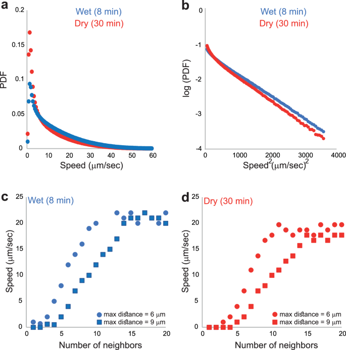
a Data presented for all speeds. Differences are mostly apparent at small speeds. b Data shown for speeds larger than 7 μm/s suggest similar distributions with Gaussian tails. c, d The average instantaneous speed of individual cells as a function of the number of their neighbors up to a cutoff distance “max distance”, (c) for the wet and (d) dry cases. Cells that do not have any close neighboring cells do not move. Then, the average speed increases with the number of neighbors up to a maximum of approximately 20 μm/s.
In Fig. 4 we compare results obtained under different illumination techniques. At a large enough frame rate (50 frames/s), when the cells are not smeared due to their motion, the fluorescence mode, the bright-field and the phase-contrast, all show that both the stationary cells and the moving ones exhibit a similar intensity, where it is impossible to tell by a single snapshot which cells are stationary, and which ones are moving. However, the DIC image shows that stationary cells and moving ones have a different color (Fig. 4d). In DIC the color (e.g., the hue of the color obtained in the HSB color system), indicates a slope in the surface of the sample with respect to the parallel microscope table (i.e., perpendicular to the beam)56. The same hue is obtained for regions in the agar that are free of cells, and for the moving cells. This suggests that the local surface of the moving cells is parallel to the agar, presumably due to the presence of a thin liquid layer on top of them, causing the cells not to be easily resolved. However, stationary cells are nicely resolved, and their hue reflects the slopes of their rod-shaped structure.

We compare four different techniques using (a) fluorescence, (b) brightfield, (c) phase-contrast, and (d) DIC. Yellow arrows indicate temporarily immobile cells, and pale-blue arrows indicate moving cells. Only DIC (d) reveals the temporarily immobile cells at even a high frame rate (50 frames/s; exposure time = 0.02 s).
To increase the DIC hue-contrast even more (Fig. 5a), we have added an additional Rochon prism to the DIC system, and then threshold the image by the hue (we “label” all pixels with hue equal or smaller than 20 in black, in between 21–24 blue, and 25–27 in green, while the agar background, as well as the moving cells are typically in the range of 43-45). Also, there are very few pixels in the entire field of view in the range of 28–42 so that the moving cells and the stationary ones are clearly distinguished (Fig. 5b). Figure 5c–g show the gradual stopping process of a single cell. Figure 5c shows a moving cell, that then stops (Fig. 5d), and starts losing the liquid around it (Fig. 5e–g), with more regions of the cell appear to be blue and black, indicating the loss of the liquid that was covering it. Figure 5h–l show the gradual acceleration of a single cell (from stationary to moving). Figure 5h–j show a stationary cell that gets wetter as the blue and black colors disappear. In the next frame (Fig. 5k), the cell is not moving yet. It eventually accelerates (Fig. 5l) as enough of the liquid covers it. Additional results (Supplementary Movie S1 and Supplementary Movie S2) show tiny ( ~ 0.5 μm in diameter) MgO beads deposited on the colony (See methods in Refs. 35,57). While beads on the virgin agar are immobile (Supplementary Movie S1), those near stationary cells (Supplementary Movie S2) do move, indicating the presence of liquid streams that are sufficient to drag the beads but not the cells. This establishes that liquid flow around a cell is not sufficient to move it.

a The field of view shows different colors (hues) that depend on the topography of the specimen. b Each pixel in (a) gets a new easy-to-follow-color (green, blue, black) based on its original hue-value. c–g A moving cell stops, and its color changes from green to black, indicating that the original hue-value changes, suggesting that the topography of the sample is different due to the lack of liquid (time intervals from the first image are indicated in the other images). h–l A temporarily immobile cell starts moving, and its color changes from black to green, indicating that the original hue-value changes, suggesting that the topography of the sample is different due to the presence of liquid (time intervals from the first image are indicated in the other images).
Next, we study the flagellar arrangement using fluorescence staining of the live bacteria (see the Methods section for details). The results show that swarming cells may be largely divided into three categories (Supplementary Movie S3). This classification is independent of the drying time. (i) Closed (Fig. 6a); with all flagella tightly wrapped around one of the poles, (ii) (Fig. 6b) Partially open; with flagella partially unbundled, and (iii) (Fig. 6c) Open; where the flagella are completely unbundled, but are still rotating. Analyzing the trajectories of the cells, the state of the flagella is labeled manually. We obtain the probability distribution of two characteristics for each of the categories. In Fig. 6d we show the distribution of speeds for the wet case (the drier case is qualitatively similar). Cells with completely unbundled (open) flagella (data in red) are almost never moving, while cells of the two other states do move, but with different speed distributions (inset of Fig. 6d). We also show the time durations the cells spend in each state (Fig. 6e). The data of the stationary cells is compared to the data taken from the DIC experiments with a fair similarity. We refer to the closed flagella state as “run”, to the partially open (partially unbundled) state “tumble”, because cells change their direction of motion and do not move in straight lines, and to the open flagella “stall”.

a–c Two examples; (a) Flagella are closed; all flagella tightly wrapped around one of the poles, (b) flagella are partially open (partially unbundled), and (c) flagella are open. Scale bar equals 10 μm. d Correlation between flagellar arrangement and cell speed. The distribution of speeds: cells with completely unbundled (open) flagella (data in red) are almost never moving, while cells in the two other states do move, but with different speed distributions (inset). e The distribution of time durations for which cells remain in a state. The distributions are practically the same for closed (green) and partially open (yellow) cells, but times are significantly longer for cells with open-flagella (red). Averages are 0.25 s for the closed, 0.21 s for the partial, and 0.95 s for the open. The distribution of the time duration in the open-flagella state, taken from the DIC experiment is superimposed (dashed black). f A histogram of the waiting times in the closed and partially-open states on a semi-log plot along with the maximum likelihood fit to an exponential distribution (averages 0.25 s and 0.21 s, respectively). g A histogram of the waiting times in the open state. The dashed and full lines show fits to a single and mixture of two exponential distributions (average 0.95 s). h The transition matrix between the states. i The two-step transition matrix. j The square of the single step one in (i). The two are equal up to a relative error of ~1%. Overall, we conclude that the transition dynamics between the states is consistent with a memoryless (continuous time) Markov chain.
Lastly, we establish that the transition between the three flagellar states is statistically consistent with a continuous time Markov chain. Figure 6f shows the histogram of the waiting times in the closed and partially open states on a semi-log plot along with the maximum likelihood fit to an exponential distribution. The fit, with averages 0.25 s and 0.21 s, respectively, is very good. Fitting the duration of the closed state (Fig. 6g) to an exponential distribution (average 0.95 s), is not as good. Fitting to a mixture of two exponential distribution is better, but is not statistically justified AIC of a single exponential – AIC of mixture = -2.5). Thus, within the data available, the approximation to an exponential waiting time is justified. Figure 6h shows the transition matrix between the states. No events of shifting directly from closed (run) to open (stall) or vice versa were observed ( > 1000 measurements). The transition from the partial (tumble) state to run or tumble are close to equal. In order to see if these transitions are memoryless, we compare the two-step transition matrix (Fig. 6i) with the square of the single step one (Fig. 6j). The two are equal up to a relative error of ~1%. Overall, we conclude that the transition dynamics between the states is consistent with a memoryless (continuous time) Markov chain whose transition probabilities are found in Fig. 6h and transition rates out of the closed, partial and open states are 4, 4.76 and 1.05 1/s, respectively.
Discussion
It is well known that moisture is a prerequisite for swarming in all bacterial species. This understanding, which has been noted since the first, pioneering works on bacterial swarming7,55,58 concerns the overall environment of the colony. In other words, it is a global requirement.
In the current work, we address the spatial and temporal local conditions for cell movement within a swarm. We showed that while clusters of cells migrate rapidly on the agar, cells in the swarming state with no close neighbors do not move until they are covered with enough liquid. Our results show that the overall availability of water plays a significant role in determining the fraction of temporarily immobile cells among a population, and the duration each of these cells will be stationary. We also see that cells that were not trapped by the local depletion of liquids are not affected and will move with similar statistics, regardless of the overall availability of the water. In addition, we show that flagellar arrangement is strongly correlated with the cellular motion, which is also strongly correlated with the local presence of liquid around the cell. Cells that are temporarily left alone are immobile, are not covered with enough liquids, and have their flagella widely open. Cells in a cluster are mobile, are covered with liquid, and have their flagella arranged in a bundle. With that, our results cannot conclude on what is the cause and what is the effect. The transitions between the flagellar states are consistent with a continuous time Markov chain.
Previous works showed that during swarming, the chemotaxis mechanism is suppressed17,59. However, cells do change direction through spontaneous clockwise flagellar rotations. This is true even in cheB mutants (B. subtilis strain DS90) that are locked in the counter clockwise direction and are constantly in a run-only phase when in liquid bulk (but not on agar)39,59. Thus, the complete opening of the flagella while stalling is not necessarily related to chemotactic behavior. These dynamics are similar to previously reported observations by Turner et al.60, who noted that Escherichia coli swarm cells follow four kinds of tracks (modes) that strongly depend on the flagellar arrangement: stalls, reversals (not studied here), lateral movement, and forward movement. The “stall” mode, which is similar to the one reported here, was mostly found in cells that are at the edge of the colony. Moreover, these cells have their flagella completely spread out, pointing outward60. They speculated that this is a mechanism for extracting or pumping water from the substrate, thus moving the colony edge forward. Our results on B. subtilis show that the completely open flagella state is also observed inside the active swarm among solitary cells that have a temporal depletion of liquid around them. This suggests that the “stall” state may be related to a cellular mechanism for extracting liquid.
Overall, we showed that moisture and the local amount of liquid around cells play a pivotal role in understanding the biophysics underling the bacterial swarming phenomenon. Specifically, dry models of self-propelled agents, which only consider steric alignments and neglect hydrodynamic interactions and the local amount of liquids, are oversimplified and are not sufficient to describe swarming bacteria.
Methods
TL DIC microscopy
In the current work we use Transmitted-Light Differential Interference Contrast (TL DIC) microscopy equipped with color “enhancement”. As in all color-DIC systems, the incident light travels through a polarizer, a Rochon/Wollaston/Nomarski prism that splits the ray, and a lambda plate. In our case, the light hits the sample from below, the bottom side of the sample is flat and smooth, and the substrate does not have birefringent properties (the bottom of the Petri-dish is made of a special glass and not the standard plastic).
Loosely speaking, the color-DIC system can differentiate between slopes in the sample, which are manifested in the hue property of colors. Differences in the index of refraction between the cells and the water (liquid), which are typically smaller than 0.05, do not play a role in determining the obtained hue, specifically in our systems where the cells are thin; Within the tested range, the same hue will be obtained for all objects in the sample if they have the same slope. In non-color DIC for instance, the differences in the index of refraction are resulted in an almost complete destructive interference, and only the perimeter of the cells may be resolved. This means that in color-DIC, cells embedded in water are almost invisible (in contrast e.g., to phase-contrast microscopy where cells embedded in water are nicely resolved).
Overall, within the experimental conditions and range of the slopes measured, the obtained hue is a monotonic function of only the local slopes in the upper surface and not of the material through which the light is transmitted. Mind that the saturation and luminance do depend on the material (its thickness or density for instance) through which the light is transmitted so the cells may sometimes be seen e.g., in Fig. 4c.
The lateral resolution (in the viewing plane) of DIC is of the order of the wavelength i.e., ~0.5 μm (stemming from the 0.2 μm adjutant points of the two split rays), and the ability to resolve the vertical axis by the hue is typically of the order of 0.05 μm, which yields an approximate minimal “local” angle of detection of ~4° (i.e., slopes smaller than 4° are not easily resolved; there is also a maximal angle above which the light is reflected away from the lens and the sample becomes dark).
In order to relate between the liquid around a cell and the measured hue value, consider a cross section of a bacterium with a cylindrical shape with a diameter 1 μm, resting on a flat surface (see Fig. 7a). Liquid (e.g., water) may cover the cell completely or partially. In Fig. 7b, the cell is completely covered. The height of the water is not important – only the angle it creates with respect to the tangent to the “ridge” of the cell. Thus, all samples that are covered by a flat-water interface will yield the same hue, regardless of the water height. In Fig. 7c we show a different case where the liquid does not completely cover the cell, resulting in different interfacial slopes around the cell. The ridge of the cell is parallel to the background and will yield the same hue. However, the edges of the cell are covered with liquid that creates a changing slope; the local slope will yield a hue that reflects the slope’s value. In Fig. 7d-e, the layer of liquid is shallow, or there is no liquid at all. In these cases, only the ridge of the cell has a parallel surface that will yield the same hue as the one seen for the background. The edges of the cell will have different hues depending on their local slopes, independently of the liquid. Upon increasing the liquid layer, the system transitions from Fig. 7d, e to Fig. 7c or even Fig. 7b, and the slopes of the liquid on the cell edges become moderate, which changes the hue to the background value. Note that the ridge of the cell is very narrow; it is narrower than the lateral resolution – therefore, the background hue is seldom obtained on the ridge.

a No liquid (b) liquid covers the cell completely (c) liquid covers cell completely with a non-uniform slope (d) shallower liquid layer with steeper angles compared to c (e) liquid layer is very shallow.
To illustrate how DIC works on transparent objects embedded in transparent medium, we performed an experiment described next and documented in Fig. 8. In Fig. 8a we show a set of 10 images of spherical silica beads (the larger ones are 5 μm in diameter) deposited on an agar surface. A drop of water, mixed with surfactant, is allowed to spread over the agar. The surfactant is added to form a relatively thin liquid front. The phase-contrast images are presented in order to show the advancing edge of the drop that covers the beads (from left to right). The images show that the beads are nicely resolved with, and without the water on top of them, and that they are not being flashed by the liquid (they are slightly embedded in the agar and a slight motion might be detected as the agar is rewetted). The 10th image shows the agar after the focus was readjusted manually. The DIC set of 10 images (Fig. 8b), shows a silica bead and the different colors (hues) that are exhibited along a diagonal line parallel to the beam splitting direction (from top-left to bottom-right). The hues reflect the structure of both the bead and the surface on which it is deposited. The top of the bead has the same hue as the one seen at the background (pale-blue). At t = 0 s, the intensity of the outer regions of the bead are low due to the relatively large angles, as most light is reflected away from the objective lens. The reddish and yellowish colors along the beam splitting direction, but outside of the bead, indicate that the bead is slightly embedded in the agar. When water approaches (from top right to bottom left), the bead is completely covered with water, and the surface becomes flat and smooth and almost parallel to the agar (except for the advancing contact angle which is very small ~ 7° (at t = 10 s); it thus appears brown and not pale-blue). In contrast to the phase-contrast case, in the DIC images the bead is completely invisible – even though we travel with the stage to find the appropriate focus. After a few minutes (the process is gradual but may be fairly seen after few minutes), the surface becomes pale-blue again because the angle of the drop decreases. The experiment lasts about 20 min during which the water evaporates and absorbed by the agar (and the bead drifts a bit with respect to the lab because the soft agar is not stable enough during the “flood”). During capturing, we play with the focus every few seconds to verify that the bead cannot be detected. The bead sometimes appears as a pale ring with a dot at its center, but only when the water level is low enough, the colors reappear.

a Phase-contrast microscopy of silica beads covered by a thin water layer. Scale bar equals 10 μm. Silica beads are placed on the agar, then water flows (see front approaching from left at t = 0.04 s). Starting at t = 0.32 s, focus is off due to the difference in height and index of refraction. Eventually, after ~8 min, the focus is readjusted manually to obtain a nice image (the water layer is still there). b DIC microscopy of silica beads covered by a thin water layer. Scale bar equals 10 μm. Silica beads are placed on the agar, the water flows from upper-right to bottom-left (see the brownish color at t = 0.02 sec), then the water covers the bead. With time, the color changes as the water levels changes its slope (with respect to the agar; blue=parallel to the agar; brown=a significant apparent slope). After ~16 min the bead reappears as the water becomes shallower.
Flagella staining
Our protocol is similar to other protocols recently used to stain flagellar filaments in Bacillus subtilis 3610 and other species60,61; yet, in our case the cells are swarmers. In the strain we have used (DS1916, amyE::Phag-hagT209C spec), the flagellin protein genes have been modified to include the cysteine amino acid that binds to the maleimide functional group62, allowing staining using Alexa 546 dye (ThermoFischer ref A10258). Bacteria are grown overnight ( ~ 18 h) in 2 ml of LB (25 g/l), at 30 °C and shaking (200 rpm), from which 10 µl is used to inoculate three swarm plates (LB with 0.5% agar). When the droplets dry out, the plates are placed in an incubator at 30 °C with controlled high humidity ( ~ 95% RH). Additionally, a fourth plate is inoculated with a one-hour delay. This plate will be used to reincorporate the stained bacteria into swarming conditions. To facilitate that process, the inoculation is done slightly off-center. The remaining overnight culture is centrifuged for 3 min at 2000 g, and the supernatant is saved for later.
The three initial plates are incubated for 5 h, after which the bacteria are collected by flushing the colonial edge with phosphate buffer (0.01 M ph~7.2) and then collecting the liquid with the cells. Special attention must be put into collecting bacteria exclusively from the edge, where bacteria are in the swarming state. If not, bio-aggregates are created by bacteria in the biofilm, disturbing the following steps. After collection, flagella are stained by adding 5 μl of the dye solution (20 μg/μl of Alexa 546 in DMSO). We allow staining to occur for one hour while the suspension is rotated at 100 rpm to prevent bacterial sedimentation. Then, bacteria are centrifuged for 3 min at 2000g and resuspended in the overnight supernatant (0.2 μm filtered). Then, 20 μl is inoculated into the fourth agar plate. The inoculation drop is introduced outside of the colony, and then it spreads along the boundary of the colony, forming an arc, never being in direct contact with the colony. After drying, the plate is replaced in the incubator for 30 min or until the colony integrates with the stained bacteria. At the end of this process, one will obtain a swarming colony where a fraction of the cells has stained flagella.
Observation was done using the same fluorescence setup described above (Zeiss Axio Imager Z2 at 63×, filter set 20 Rhodamin shift free: Excitation 546/12; Beam Splitter 560; Emission 607/80), and a Zyla Andor operated at 100 frames per second.
Image analysis
The quantitative analysis presented in Figs. 2 and 3 is facilitated using custom image analysis software implemented in Matlab. First, images undergo standard smoothing and preprocessing, as detailed in Ref. 40. Applying a threshold on the intensity yields a Boolean mask indicating whether each pixel corresponds to a cell or not. Occupancy statistics (Fig. 2) corresponds to pixel-wise counts (and not number of cells).
The sequence of images is used to obtain velocity field using optical flow analysis (see30 for details). Such algorithms inherently involve smoothing. Average speeds (Figs. 3a, b) are obtained directly from the vector fields without taking into account speeds below a threshold. In other words, we average only over pixels that correspond to moving objects. The implementation follows40.
Figure 3c, d show the average speed of cells as a function of the number of neighbors (up to a given distance). This requires identifying the position of individual cells and therefore tracking of individuals. To this end, we apply a method for tracking elongated objects using the Hough transform. First, the Boolean mask is separated into connected blobs using standard image analysis tools in Matlab. Blobs that are too small (in area or length) are discarded. The main difficulty is that cells that are practically touching are often associated with the same blob. To bypass this problem, in each blob, we find the longest line segment using the Hough transform. This segment (with some added thickness) is removed from the blob. Segments that are longer than 1.5 the average cell length are split in two. Repeating the process, we obtain a list of line segments that correspond to the individual cells.
Once individual cells were identified as line segments, we need to associate cells in consecutive frames to obtain trajectories. Typically, tracking software use the central points to find which cell in one image is closest to which cells in the following one. Here, we use the sum of the distances between the endpoints, which also takes into account the orientation and length of the detected cells. Since the order of the endpoints in each line segment is arbitrary, one needs to take the minimum between two ordering options. We perform a standard greedy pair matching algorithm, starting at the closed pair up to a cutoff distance of about 3 average cell lengths.
Next, the endpoints of each trajectory are smoothed over time using malowess with a linear interpolation. Velocities of the center of mass can then be calculated. Finally, to calculate the number of neighbors a focal cell has up to a given distance, we find the average number of endpoints associated with other cells to each of the endpoints of the focal cell. In other words, instead of counting cells, we count endpoints, each “worth” half a cell. This counting is used to calculate the statistics in Fig. 3c, d.
Reporting summary
Further information on research design is available in the Nature Portfolio Reporting Summary linked to this article.
Responses