Importance of the vertical mixing process in the development of El Niño Modoki

El Niño/Southern Oscillation (ENSO) is the most dominant interannual climate mode significantly affecting global climate through teleconnections^1,2. It displays considerable variability across events and it is often categorized into two groups according to the location of maximum sea surface temperature (SST) anomalies^3,4. Canonical El Niño events are associated with the maximum anomalous warming in the eastern equatorial Pacific, whereas positive SST anomalies peak in the central equatorial Pacific and negative SST anomalies develop in the western and eastern equatorial Pacific during El Niño Modoki events^5,6. The latter El Niño type with positive SST anomalies in the central Pacific is also referred to as the central Pacific El Niño⁷, the date line El Niño⁸, and the warm pool El Niño⁹. These different flavors of ENSO received considerable attention recently, as their remote influences are quite different^8,10 and their occurrence frequency¹¹ may change under the influence of global warming^12,13,14,15, although ENSO diversity may also be intrinsically modulated^16,17,18.

Not only the spatial pattern of SST anomalies, but also the mechanisms responsible for generating positive SST anomalies are considered markedly different. While the vertical processes are considered to contribute dominantly to the development of canonical El Niño^19,20,21, the zonal advection of the mean zonal temperature gradient by anomalous zonal current, also referred to as the zonal advective feedback, has been suggested to play an important role in the formation of positive SST anomalies in the central equatorial Pacific during El Niño Modoki^9,16,20,22. The importance of the zonal advective feedback in the central equatorial Pacific is partly due to the strong mean zonal SST gradients near the eastern edge of the western Pacific warm pool, and partly due to relatively smaller vertical excursion of the thermocline on ENSO time scales compared to the eastern equatorial Pacific. Moreover, downwelling Kelvin and Rossby waves induced by equatorial zonal wind stress anomalies⁵, the wind-evaporation SST feedback from the subtropical Pacific²³, and the upper layer convergence driven by anomalous winds have been suggested to contribute to the anomalous SST warming²⁴. However, these past studies on El Niño Modoki overlooked the contribution from vertical mixing. Due to the strong vertical current shear between the South Equatorial Current flowing westward near the surface and the Equatorial Undercurrent (EUC) in the subsurface flowing eastward²⁵, active turbulent mixing is observed in the upper ocean of the equatorial Pacific^26,27,28,29.

Here the generation mechanisms of positive SST anomalies in the central equatorial Pacific associated with El Niño Modoki is quantitatively investigated by conducting a mixed layer heat budget analysis using outputs from a hindcast simulation of a regional ocean model configured for the tropical Pacific (see “Methods”).

Evolution of El Niño Modoki

In this study, the observed El Niño Modoki index (EMI; see “Methods”) is used to identify six El Niño Modoki events (1967, 1977, 1991, 1994, 2004, and 2009) (Supplementary Fig. S1). To examine the evolution of SST anomalies associated with El Niño Modoki and validate the use of the regional ocean model, Fig. 1 compares composites of observed and simulated SST anomalies associated with El Niño Modoki events. In April-June (AMJ) (0) (see “Methods” for the naming convention of years in parentheses), weak positive SST anomalies first appear just to the east of the date line. These SST anomalies expand and amplify in July-September (JAS) (0) and peak in October-December (OND) (0) with the peak SST anomalies centered between 180° and 150°W. Then, SST anomalies start to decay in January-March (JFM) (1) and equatorial SST anomalies almost completely disappear by AMJ (1). The model is generally successful in reproducing the evolution of positive SST anomalies associated with El Niño Modoki, although the peak SST anomalies in OND (0) is slightly underestimated.

Composites of SST anomalies in a, b April–June (AMJ) (0), c, d July–September (JAS) (0), e, f October–December (OND) (0), g, h January–March (JFM) (1), and i, j AMJ (1) for El Niño Modoki events based on (left) HadISST and (right) ROMS. From top to bottom, the temporal evolution is divided into five seasons. Anomalies significant at the 95% confidence level by a two-tailed t test are shaded.

Full size image

Generation mechanisms

To quantitatively investigate the generation mechanisms of positive SST anomalies in the central equatorial Pacific associated with El Niño Modoki events, composites of monthly anomalies for each term in the mixed layer heat budget equation (see “Methods”) are prepared from January (0) to October (1) that covers both development and decay phases (Fig. 2).

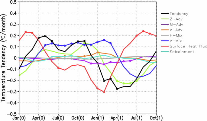
Composite of the 3-month running mean monthly anomalies for each term in the mixed layer heat budget analysis equation averaged over the central equatorial Pacific (165°E-140°W, 1°S-1°N) for El Niño Modoki events. Anomalies of mixed layer temperature tendency (black), zonal advection (Z-Adv, yellow green), meridional advection (M-Adv, purple), vertical advection (V-Adv, orange), horizontal mixing (H-Mix, gray), vertical mixing (V-Mix, blue), surface heat flux (red), and entrainment (light blue) terms from January (0) to October (1) are plotted. Dots indicate anomalies significant at the 95% confidence level by a two-tailed t-test.

Full size image

The mixed layer temperature tendency anomalies are positive from February (0) to December (0), with statistically significant anomalies during April (0)-June (0) and October (0)-November (0). The surface heat flux term significantly contributes to the development of positive SST anomalies in February (0) and March (0), although the positive anomalies in the tendency term remain statistically insignificant. When decomposed into four components (Supplementary Fig. S2), shortwave radiation and latent heat flux anomalies are the primary contributors to positive anomalies in the net surface heat flux, though these contributions are also not statistically significant. From May (0) to March (1), it is the vertical mixing term that contributes most consistently throughout the development phase with statistically significant positive anomalies. Given that the net effect of the vertical mixing is to cool the mixed layer, this suggests that the anomalous warming is caused by a suppression of the cooling by vertical mixing. The magnitude of the anomalous vertical mixing term, however, is much smaller compared to the eastern equatorial Pacific, where the anomalous vertical mixing term is an order of magnitude greater²¹. The zonal advection also contributes to the development of positive SST anomalies, but it is statistically significant only in November (0) and its amplitude is about a half of the vertical mixing term in the composite. The dominance of the zonal advection term over the vertical advection term is consistent with past studies^9,16,20, but this study points out the importance of the vertical mixing term. On the other hand, the surface heat flux term turns anomalously negative from June (0) and operates as a negative feedback, especially in January (1) and February (1), when the positive SST anomalies start to decay. This is primarily due to negative shortwave radiation anomalies linked to an increase in atmospheric deep convection above positive SST anomalies as well as enhanced heat loss from latent and sensible heat fluxes associated with positive SST anomalies. After April (1), the zonal advection term contributes significantly to the decay of positive SST anomalies. Also, the meridional advection term weakly but significantly contributes to the damping of positive SST anomalies from December (0) to June (1).

To examine how the relative importance of different terms varies across El Niño Modoki events, I have integrated each term during the development phase of each event (see “Methods”). As shown in Fig. 3, the contribution from the vertical mixing term dominates over that from the zonal advection term in three events (1967, 1994, and 2004), and the contribution from the zonal advection and vertical mixing terms are comparable in the 1991 event, while the zonal advection term contributes dominantly in the 1977 and 2009 events. Thus, the vertical mixing term makes a dominant or comparable contribution to the anomalous zonal advection term during the development of El Niño Modoki in four out of six simulated events.

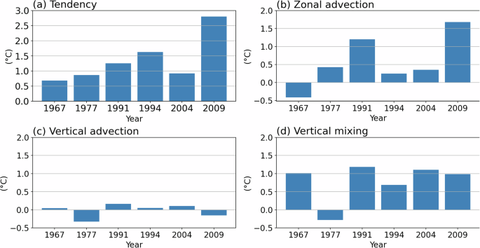
a Tendency, b zonal advection, c vertical advection, and d vertical mixing term anomalies in the central equatorial Pacific (165°E–140°W, 1°S–1°N) integrated over the development phase (see “Methods”) of El Niño Modoki events (in °C).

Full size image

The qualitative results are not very sensitive to a slight shift in the box region. For example, when the equatorial strip of the Niño-4 region, which is often used to define the central Pacific El Niño⁷ and located slightly to the west of the region used to compute the El Niño Modoki index, is used, the vertical mixing remains the primary term (Supplementary Fig. S3), although the magnitude of the vertical mixing and zonal advection terms become more comparable as the box is shifted westward (Supplementary Fig. S4). The weaker contribution of the vertical mixing term towards the west may be due to weaker vertical shear between the surface South Equatorial Current flowing westward and subsurface Equatorial Undercurrent flowing eastward. Also, barrier layers more often develop in the west^29,30,31,32, inhibiting mixing of cold subsurface water.

Decomposition of the vertical mixing term

To gain further insight into the anomalous vertical mixing term, the vertical mixing term is decomposed into the contributions from the vertical heat flux and mixed layer depth (MLD) anomalies (see “Methods”). By estimating their contributions (Fig. 4), it is found that the contribution from the vertical heat flux anomalies dominates over that from MLD anomalies.

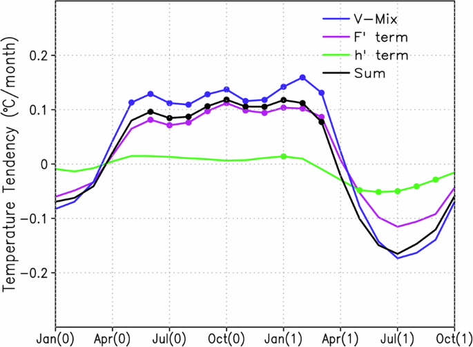
Composites of anomalies in the vertical mixing term (V-mix; blue), the contribution from vertical heat flux anomalies (({F}^{{prime} }) term; purple), the contribution from MLD anomalies (({h}^{{prime} }) term; green), and the sum of ({F}^{{prime} }) and ({h}^{{prime} }) terms (black) (see “Methods”). Dots indicate anomalies significant at the 95% confidence level by a two-tailed t-test.

Full size image

To explore the mechanisms of anomalous vertical heat flux associated with vertical mixing, vertical temperature gradient and diffusion coefficient anomalies are examined (Fig. 5). Vertical temperature gradient anomalies around the base of the mixed layer are negative in the central and eastern equatorial Pacific, signifying that the vertical temperature gradient is slackened. This is associated with anomalous deepening of the thermocline. Although the anomalies are stronger toward the east, anomalously weak vertical temperature gradient is also found in the central equatorial Pacific. Since the vertical temperature difference across the mixed layer base is anomalously small, the vertical mixing process is less efficient in cooling the mixed layer and contributes to the anomalous warming. Furthermore, vertical diffusion coefficient anomalies are also negative near the mixed layer base, especially between 150°E and 180°. These negative anomalies also favor weaker cooling by the vertical mixing process, and are associated with weaker vertical shear between the surface South Equatorial Current flowing westward and subsurface Equatorial Undercurrent flowing eastward (Supplementary Fig. S5).

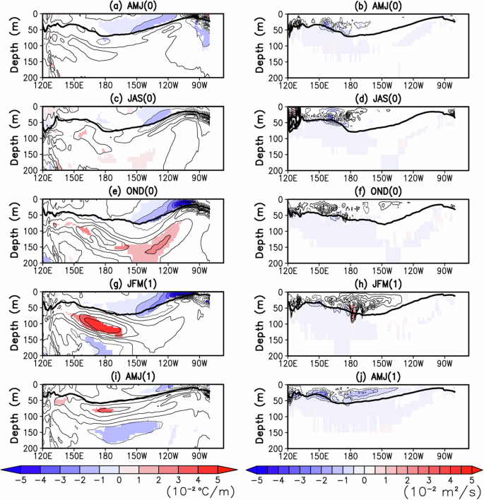
Composites of vertical (left) temperature gradient and (right) diffusion coefficient anomalies along the equator in a, b AMJ (0), c, d JAS (0), e, f OND (0), g, h JFM (1), and i, j AMJ (1) for El Niño Modoki events. Anomalies significant at the 95% confidence level by a two-tailed t-test are shaded. The contour intervals are 0.01 °C/m and 0.005 m²/s for the left and right columns, respectively. The thick black lines indicate the mixed layer base.

Full size image

It has long been considered that the zonal advection term plays a key role in the development of El Niño Modoki^9,16,20, but it is shown for the first time that the vertical mixing process also makes an important contribution in El Niño Modoki events. However, since the present study relies solely on an ocean model simulation, which is affected by model biases, including those arising from uncertainties in vertical mixing parameterization, the main findings need to be validated with observations. Currently, there is only one sustained turbulent mixing measurement in the equatorial Pacific at 140°W, but this is located on the eastern edge of the box region that I have conducted a heat budget analysis. To verify that the vertical mixing plays an important role in the development of the positive SST anomalies during El Niño Modoki, a sustained measurement of turbulent mixing further to the west is needed.

Also, it was previously speculated that an increase in the frequency of El Niño Modoki under global warming is related to the flattening of the east-west tilt in the equatorial thermocline that leads to shoaling of the thermocline and an enhanced zonal advective feedback in the central equatorial Pacific¹². The present finding that the vertical mixing process plays an important role in the development of El Niño Modoki suggests that future changes in ENSO may be closely linked to that in vertical mixing. Thus, further studies on possible future changes of El Niño Modoki from the new viewpoint may be worthwhile.

Regional ocean model

I use a hindcast simulation²¹ based on the Regional Ocean Modeling System (ROMS)³³ configured for the tropical Pacific (120°E-67°W, 25°S-25°N). Its horizontal resolution is 0.25° in both zonal and meridional directions, and there are 40 vertical sigma levels. After the model was spun up for 20 years, it is integrated for 59 years (1958–2016) with the daily atmospheric and river data and the monthly lateral boundary conditions. For the former, the daily Japanese 55-year atmospheric reanalysis (JRA55-do)^34,35 is used, while the monthly Ocean Reanalysis System 4 (ORAS4)³⁶ is used for the latter. All the model outputs were stored as 5-day mean and the outputs from the last 56 years (1961–2016) are used in this study.

Observational and reanalysis data

For the model validation, the Hadley Centre Global Sea Ice and Sea Surface Temperature (HadISST)³⁷ dataset from 1961 to 2016 is used. Its horizontal resolution is 1° × 1°. In addition, the ORAS4 product³⁶ for the same period is used for the validation of simulated subsurface oceanic variables. The horizontal resolution is 1° × 1°, and there are 42 levels in the vertical direction.

El Niño Modoki years

To identify El Niño Modoki years, I use the EMI⁵, which is defined by

where ({{SSTA}}_{A}), ({{SSTA}}_{B}), and ({{SSTA}}_{C}) represent area-averaged SST anomalies over (165°E-140°W, 10°S-10°N), (110°W-70°W, 15°S-5°N), and (125°E-145°E, 10°S-20°N), respectively. The EMI obtained from HadISST and ROMS is highly correlated with their correlation coefficient equals 0.92. When the EMI in OND obtained from HadISST is greater than +1σ, the year is defined as El Niño Modoki year. In the case of two consecutive years of El Niño Modoki events (i.e., 1990 and 1991), I only select the latter year, although qualitative results are not sensitive to this selection. As a result, six El Niño Modoki events (1967, 1977, 1991, 1994, 2004, and 2009) are obtained. Since the number of events is somewhat limited, results from each event are also reported for key findings in this manuscript. These years with the EMI exceeding +1σ is referred to as Year 0, and the following year is referred to as Year 1. These years will be indicated in brackets after months (e.g. December of Year 0 is denoted by December (0)). The development phase of El Niño Modoki is defined to start from the first month with positive tendency in the mixed layer temperature for at least two consecutive months and end on the first month after October (0) with negative tendency in the mixed layer temperature in Year 0.

Mixed layer heat budget analysis

A mixed layer heat budget equation^21,38,39 may be written as follows:

Here, ({T}_{{ml}}) is defined as the temperature averaged over the mixed layer, whose depth is defined as the depth at which potential density increases by 0.125 kg m⁻³ from the sea surface²¹. With this definition, SST and ({T}_{{ml}}) anomalies have extremely high correlation coefficient of 0.9994 and a root-mean-square deviation of only 0.03932 °C. When I use fixed MLD of 66.4 m, which is the mean MLD for the above density-based criterion, the correlation coefficient and root-mean-square deviation degrade to 0.9830 and 0.1867 °C, respectively, supporting the use of the above density-based definition. Also, (T) is temperature, (h) is MLD, (u) is zonal velocity, (v) is meridional velocity, (w) is vertical velocity, ({K}_{v}) is the vertical diffusion coefficient, ({K}_{h}) is the horizontal diffusion coefficient, ({w}_{e}) is the entrainment rate ((=partial h/partial t)), (Delta T) is the difference between ({T}_{{ml}}) and the temperature of the entrained water, ({rho }_{0}) is the density of the seawater (1024 kg m^-3), ({C}_{p}) is the specific heat of the seawater (3980 J kg^-1 K^-1), ({Q}_{{net}}) is the net surface heat flux, and ({Q}_{{psw}}) is the penetrative shortwave radiation at the mixed layer base.

The right-hand side contains the zonal, meridional and vertical advection terms in the first line, the horizontal mixing term in the second line, and vertical mixing, entrainment, and surface heat flux terms in the third line. Other than the entrainment term, which is diagnostically calculated based on the formulation that ensure exact closure of the mixed layer heat budget⁴⁰, each term in Eq. (2) is obtained by integrating the respective terms in the governing equation for temperature in the model vertically from the sea surface to the base of the mixed layer. As a result, the left hand side of Eq. (2) and the sum of all terms on the right hand side are exactly equal with no residuals in the present analysis.

Decomposition of the vertical mixing term

To gain insight into the anomalous vertical mixing term, the vertical mixing term in Eq. (2) is decomposed as follows²¹:

Here, a prime and a bar represent an anomaly and a climatological value, respectively, and (Res.) is a higher-order term. The first term on the right-hand side represents anomalous warming of the mixed layer temperature by anomalous vertical heat flux across the base of the mixed layer (denoted as ({F}^{{prime} }) term), whereas the second term reflects changes in the effective heat capacity of the mixed layer associated with anomalies in MLD (labeled as ({h}^{{prime} }) term).