Incomplete mass closure in atmospheric nanoparticle growth

Introduction
The formation of new aerosol particles via gas-to-particle conversion is the dominant source of ultrafine aerosol particles in the atmosphere and a major contributor to the global cloud condensation nuclei budget1. Aerosol-cloud interactions are a major source of uncertainty in climate models2 and especially model implementations of new particle formation (NPF) often lack an in-depth phyicso-chemical understanding3. Decisive for the climate impact of NPF is a high enough growth rate (GR) of the newly formed particles4. Only through fast growth, the particles can quickly escape the sub-10 nm range where they are most susceptible to scavenging by pre-existing larger aerosol particles5. At many continental sites, nanoparticle growth is dominated by the condensation of oxygenated organic molecules (OOMs) originating from the oxidation of volatile organic compounds (VOCs)4,6. However, measuring and modeling the growth from a wide variety of different organics from biogenic and anthropogenic sources is an extreme analytical challenge7. To-date most large-scale models still underestimate both the mass and number fraction of secondary organic aerosol (SOA) when compared to observations4,8.
Some studies have reported closure between the condensational growth predicted from measured gas-phase organics and the observed GRs of an aerosol population. Most of these studies still assume a kinetic condensation model without curvature or solution effects9,10. Using the measured volatility distribution, the studies reporting closure are limited for the most part to well-defined chamber experiments7,11, studies that used extensive parameter tuning12, or case studies of some spring-time NPF events in the boreal forest13, and some summer-time NPF events close to a roadside in Leipzig, Germany14. A recent comparison of GRs inferred from measured size distributions and modeled from observed organic vapors in urban Beijing could only achieve a reasonable agreement for the smallest particle sizes15. However, below 3 nm, growth is anyways often driven mainly by sulfuric acid and associated bases16,17,18. At sizes above 3 nm, results from Beijing showed significant discrepancies with lower modeled than observed GRs in winter, but better agreement in summer19.
Here, we investigate the closure between GRs derived from the particle-size distribution and calculated from measured gas-phase concentrations for three complementary measurement sites and show that obtaining mass closure is still “exceptional”. In line with previous investigations4,20,21, we find that the observed GRs range mostly between 1 and 10 nm h−1, while total condensable vapor concentrations show a much higher variability. We demonstrate that modeled GRs are often too low due to an incomplete coverage of gas-phase OOMs, which is especially important at colder temperatures. Most importantly, we also report cases where the modeled GRs exceed the observed GRs. While it is easier to invoke “undetected” vapors to explain predictions that are too low, explaining why observed condensable vapors do not drive growth is a taller challenge. These cases are exemplars illustrating the problem of the surprisingly limited GR variation observed both at single sites20,21 and across continental observations4.
Results
Limited variability in observed nanoparticle growth rates
OOMs are a key contributor to atmospheric NPF and subsequent growth4,22,23, especially when they are highly oxygenated. In the boreal forest, the majority of OOMs originate from biogenic VOCs such as monoterpenes, which can undergo rapid oxygenation by autoxidation24. The resulting highly oxygenated organic molecules25 are often measured using a nitrate chemical ionization mass spectrometer (NO3− CIMS)26. We show in Fig. 1, that the sum of gas-phase OOMs based on NO3− CIMS measurements shows a variability of about 2–3 orders of magnitude at three contrasting environments (Hyytiälä, Finland, Beijing, China, and San Pietro di Capofiume, Italy, see “Materials and methods” for details) with typically lower OOM concentrations measured during the colder seasons. In contrast, the observed organic-driven nanoparticle GRs (where the known contribution of sulfuric acid is subtracted27) mostly range between 1 and 10 nm h−1. The limited variability of observed GRs inferred from the particle-size distribution seems to be a more general feature across most measurement sites4.

The assumed contribution from sulfuric acid has been subtracted from the observed GR (GR-GR(H2SO4)). a The results for the 1.5–3 nm size range and b The 3–7 nm size range. Data from three measurement sites is shown: Hyytiälä, Finland (squares); Beijing, China (diamonds) and San Pietro di Capofiume, Italy (triangles). The color code represents the temperature. The circles show results from the CERN CLOUD experiment from pure α-pinene ozonolysis experiments at three different temperatures (−25 °C, +5 °C, +25 °C). The dashed line shows the expected GR for the case that all OOMs measured by the NO3− CIMS would condense at a rate limited only by the collision kinetics (kinetic limit).
One possibility for that limited variability is that low GRs (<1 nm h−1) are typically not detected due to limited sensitivity towards low number concentrations28 and that high GRs (>10 nm h−1) are missed due to limited time-resolution of size-distribution measurements29. However, it was recently estimated that nanoparticles are growing at similar GRs also during non-NPF event days with low counting statistics (no clear growing mode and only a few counts per size-interval) in the sub-10 nm particle size-distribution measurements30. In addition, long-term trends show an increase in average OOM concentrations31, mainly due to the scaling of biogenic VOC emissions with temperature. This is again not reflected in observed GRs as shown in Fig. S1 in the SI Appendix, even if that increase would be expected to be within the range of “robust” GR estimates (i.e., 1–10 nm h−1). Altogether, this raises the question if the limited variation in GRs can be attributed to curvature-, solution-, and temperature effects, or if larger measurement uncertainties or unaccounted physico-chemical processes are present.
For the smallest size range studied here (1.5–3 nm, Fig. 1a), the uncertainty in the GR estimates is much larger due to typically lower counting statistics28. In addition, the increased Kelvin barrier will hinder the condensation of OOMs at that size range22,32. Especially at warmer temperatures, many OOMs might not be of sufficiently low volatility7, and thus corresponding measured GRs are well below the expected limit of kinetic condensation of all OOMs. Overall, this results in a poor correlation between OOMs and GR, similar to earlier studies33. In the larger size range (3–7 nm, Fig. 1b), the GR measurement uncertainties are lower, and a significant fraction of the NO3− CIMS measured OOMs should condense onto the particles as the Kelvin barrier has decreased, but even here the correlation is still low. For comparison, we also included the results from pure organic growth measurements (α-pinene ozonolysis) for three different temperatures conducted at the CERN CLOUD experiment7. These results showed that part of the variation of condensable vapors measured by NO3− CIMS is due to its high selectivity towards highly polar molecules34. Since at colder temperatures, even less polar molecules can contribute to growth7, the low NO3− CIMS-based OOM concentrations might under-represent the total condensable material, which was already speculated for Beijing19. This shows that some variation in condensable vapor concentration can be explained by the temperature-dependent shifting of NO3− CIMS sensitivity towards the actual condensable vapors.
Mass closure for springtime boreal forest nanoparticle growth
Several chamber studies11,35,36 and ambient measurements in Hyytiälä13 and Beijing19 have shown that the volatility-distribution of OOMs matters decisively for particle growth. The volatility distribution is typically defined in bins as well as broader ranges in the Volatility Basis Set (VBS) to simplify the complexity of atmospheric organics37. These studies also showed that small changes in the volatility distribution of OOMs, e.g., due to the addition of NOx or other VOCs, directly induce significant shifts in the observed particle GRs at sizes smaller than 10 nm.
To avoid the bias from unmeasured OOMs, we use a combination of two chemical ionization schemes with different reagent ions (NO3− CIMS and a Br− CIMS)38 to obtain a more complete coverage of the volatility distribution (see “Materials and methods” and Figs. S2 and S3 in the SI Appendix). Figure 2a shows that in the ranges of low-volatility organic compounds (LVOC) and extremely low-volatility organic compounds (ELVOC), the Br− CIMS adds around a factor of 2–4 in concentration to most VBS bins, with an increasing importance in the LVOC range. With the volatility distribution covered by these two complementary ionization schemes, we used a monodisperse growth model to estimate the GR expected from the gas-phase measurements39. Here, we adjusted the model to include co-condensation of sulfuric acid (see Materials and Methods for details)27. To test the sensitivity of the growth model, we applied a ±1 bin uncertainty (i.e., shifting the entire volatility distribution by one order of magnitude at 300 K), which also captures the uncertainty in the volatility parametrization (see Fig. 2c).
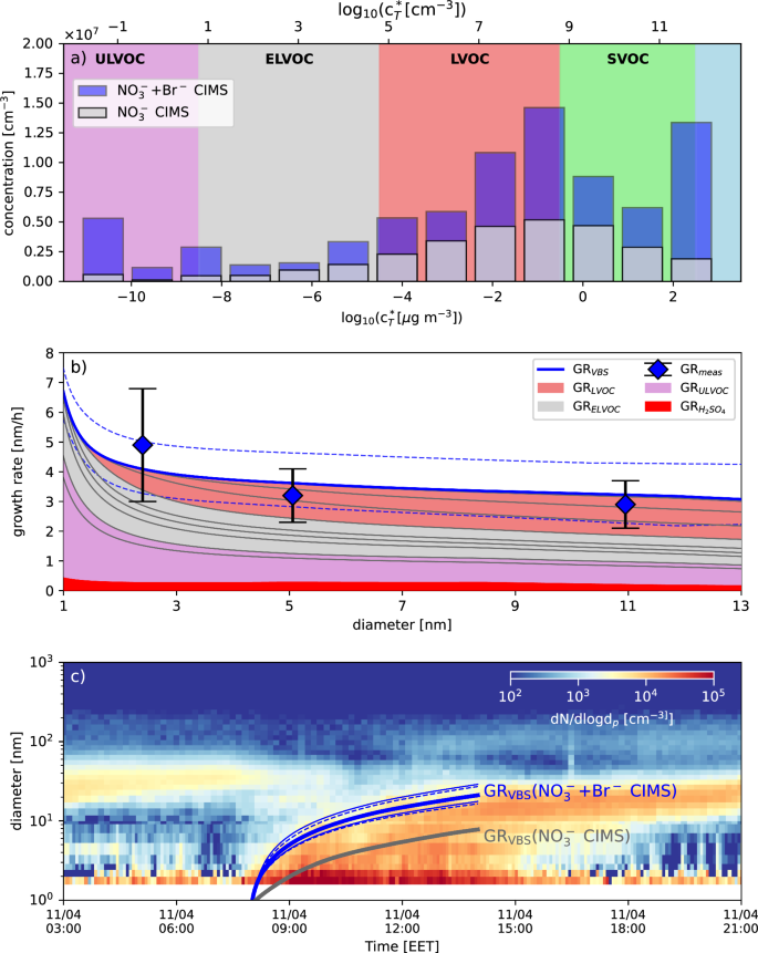
a The volatility distribution of the OOMs at the average temperature (3.8 °C) of one example NPF event day (11th April 2020). The gray bars show the volatility distribution of the NO3− CIMS only, and the blue bar shows the volatility distribution of the combined ionization schemes. b A size-dependent comparison of the observed GRs (blue diamonds) and the model-predicted GRs (blue solid line with the different colored areas indicating the contribution to GR from different vapor classes). The two dashed blue lines give the ±1 order of magnitude uncertainty in volatility assignment. c The particle size distribution evolution during the event day together with the calculated median growth from the VBS-based growth model (solid thick lines, blue for the combined ionization schemes and gray for the NO3− CIMS only) and a corresponding uncertainty estimate for the model (blue thin solid line are two alternative VBS parametrizations)7,13.
We achieve mass closure (in terms of gas-phase predicted and size-distribution observed GRs) during springtime in Hyytiälä, as shown in Fig. 2b similar to the earlier results13. Our predictions match across three different particle size ranges, which were probed with state-of-the-art particle number size distribution instruments (see “Materials and methods” for details). The model even predicts the measured decreasing GR with size for that specific day, which is a rather unusual GR size-dependency for the boreal forest40.
Figure 2c demonstrates how important it is to include the Br− CIMS in the volatility distribution. The growth trajectory calculated from the NO3− CIMS alone remains well below 10 nm in size even after several hours of growth. Moreover, the shortfall from undetected condensable material is significantly larger than the uncertainty in the volatility assignment. Consistent with the earlier results13, we can conclude that mass closure between observed gas-phase species and measured particle GRs can be achieved for springtime boreal forest conditions by assuming only gas-phase condensation without any further need for particle-phase chemistry when using dedicated ionization schemes for broad coverage of gas-phase OOMs of all oxidation states.
Slower than predicted GRs
In the summer-time boreal forest, the higher biogenic activity results in much higher biogenic VOC levels41. In addition, we expect autoxidation at higher temperatures to be more rapid7, which should result in more highly oxygenated molecules. Even though we adjust our volatility distribution for the higher temperatures in summer, where the same OOM will be typical of higher volatility compared to spring, the higher emissions and faster oxidation result in an increase in all classes relevant for newly formed particle growth, i.e., the (E)LVOC ranges, with even up to one order of magnitude higher concentrations of the decisive LVOCs (see Fig. 3a). While we typically observe higher GRs during summer-time in the boreal forest40, the increase is much smaller than the almost one order of magnitude increase in OOM concentrations across the entire volatility range relevant for growth. In fact, our growth model reveals a discrepancy in the absolute values between measured and observed GRs by around a factor of 3 (see Fig. 3b), while it identifies the typical size-dependency of higher GRs above 3 nm. This discrepancy is significantly higher than the estimated intrinsic uncertainty of the VBS method and the volatility assignment.
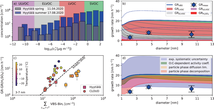
a The volatility distributions of the OOMs as measured by the combined ionization schemes at the average temperature of the two example events days, the 11th April 2020 (3.8 °C, gray bars), and the 17th August 2020 (17.5 °C, blue bars). b The model-predicted GR for the 17th August 2020 from the VBS growth model (thick blue line for total GR) versus diameter (with the different colored areas indicating the contribution of different condensable vapor classes). Blue symbols give the observed GR values and the dashed blue lines represent the model uncertainty (±1 bin shift of the entire VBS). c The observed GR (squares, again corrected for the contribution of sulfuric acid) of all analyzed NPF event days during the campaign (where both NO3− and Br− CIMS were available) versus the amount of condensable material determined by the VBS (i.e., the sum of all VBS-bins in supersaturation). Circles show the pure α-pinene reference experiments. Color code gives the average temperature of the event day (summer >10 °C, spring <10 °C) or the experiment. The dashed black line gives the expected growth rate if all the VBS bins in supersaturation condense at a rate limited only by the collision kinetics (kinetic limit). d The potential reasons for the observed discrepancy with the blue line showing the base model result and the blue diamonds the observed GR values. The blue-shaded area shows the maximum range of systematic uncertainty due to experimental quantification of the condensable vapors. The green shaded area gives the range of model results when the model is run on O:C-dependent activity coefficients. The red shaded area gives the model results when particle phase decomposition reactions (ULVOC and ELVOC dimer breakdown) are included. The yellow shaded area gives the range of the model results when particle-phase diffusion limitations due to semi-solid to solid-like particles are included.
We also observe higher predicted than measured GRs in the Po-Valley and Beijing as shown in Fig. S4 in the SI Appendix, even though these locations are complimentary in the sense that different VOCs and oxidation mechanisms are responsible for OOM formation. Only NO3− CIMS gas-phase data were available for these sites, which should generally result in a model underestimation of the measured GR. However, the observed GRs are slower than predicted GRs for some cases in Beijing summertime and even in spring-time Po-Valley. Inclusion of additional measurement schemes accounting for “hidden” OOMs is expected to even further increase that discrepancy for these sites.
Figure 3c shows a comparison of all in-depth analyzed Hyytiälä summer- and springtime events (see Table S1 in the SI Appendix) to the results from the CERN CLOUD pure α-pinene experiment. We plot the GR versus the sum of all VBS bins in supersaturation (({c}_{i,g} ,>, {c}^{0})), i.e., the VBS-derived condensable material. For CLOUD it has been demonstrated that results from different temperatures can be brought into reasonable agreement using that approach7. For Hyytiälä, we find that the spring events are well in line with the CLOUD results. The measured GRs are slightly above the kinetic limit of condensation as solution effects are unaccounted for. They lower the saturation vapor pressure of each VBS bin and hence induce significant partitioning to the particle phase also of bins not in supersaturation (typically the most volatile LVOC and the least volatile SVOC bin). However, the summer events show slower growth than the kinetic limit of condensation of all VBS bins in supersaturation. This indicates either a significant systematic uncertainty to be present in summer or a potential rate-limiting process hindering kinetic condensation of the gas-phase condensable vapors.
Probable causes for a growth-rate limiting process
The most probable experimental systematic uncertainty causing such a deviation between the observed and predicted GRs is the uncertainty in the quantification of OOMs. Our in-depth analysis focused on event days with the most robust GR estimates (see “Materials and methods” and Table S1 in the SI Appendix), avoiding too large systematic uncertainty from the size-distribution measurements. In addition, the ±1 bin uncertainty in the volatility assignment is not sufficient to explain the discrepancy. It is unlikely that deviations from the expected temperature dependence of the volatility would become evident at the warm (closer to 300 K) temperature as the volatility assignment is anchored on data at 300 K37 (see “Materials and methods” for details).
Our experimental systematic uncertainty estimate, which takes into account calibration and transmission errors for OOM quantification (see “Materials and methods” for details), can bring the model and measurement close to agreement (Fig. 3d). However, we expect our measurements to be rather a lower estimate of OOM concentrations, as OOM charging efficiencies are probably lower than assumed (as the quantification is bound to the efficient H2SO4-NO3− charging). In that sense, the largest model-observation discrepancy for the smallest particle size range is especially puzzling, as the quantification of the highly polar ULVOC and ELVOC molecules (decisive for early growth) should be closest to the H2SO4-NO3− charging. Last, the sensitivity of the instruments would need to strongly depend on external conditions not captured by the calibration procedures to explain why there is good agreement between observed and predicted GRs in spring, but not in summer. Apart from experimental uncertainties, we tested three potential microphysical and chemical processes that could cause slower GRs within our model: (1) strong interactions between the different organics in the particle phase altering their particle phase activity, (2) particle-phase reactions which would result in decomposition of ULVOC and ELVOC compounds into products of higher volatility forcing their re-evaporation from the particle, and (3) particle-phase diffusion limitation in the mass-transfer due to semi-solid to solid particles.
Interactions between the different organics in the particle phase could cause phase separation during the growth process thereby slowing it down. This is described by high activity coefficients, where we follow the explicit modeling that links the activity coefficients to differences in the O:C ratio (ΔO:C) between the condensing molecule (VBS-bin (i)) and the average of the remaining particle phase37. We show in Fig. 3d that there is no effect on the GR if the non-linearity coefficient of the (bulk-property-based) 2d-VBS is used (see Materials and Methods for details). Only if the coefficient is increased by more than two orders of magnitude the GRs slow down. However, the observed GR and especially their size-dependency cannot be reproduced by the model and such a strong ΔO:C-activity coefficient relation is in contradiction to other results for large-scale particles42, which only found SOA phase separation at ΔO:C > 0.5. Our growth model would require activity coefficients >5 already at ΔO:C(sim)0.06 for the GR to be significantly slowed down, but it is theoretically possible that phase separation occurs earlier on the nanoscale43,44.
Particle phase reactions which would decrease O:C of all condensed phase organics gradually, e.g., decarboxylation (CO2 abstraction)45 or loss of H2O through e.g., Baeyer–Villiger reactions46, would slowly shift molecules from VBS bins with lower volatility toward VBS bins with higher volatility. Breaking of ULVOC and ELVOC dimers could also slow the GR47. For simplicity, we adjusted our model to assume that all ULVOC and ELVOC bins are composed of dimers, which all break at the same rate (see “Materials and methods” for more details). That way, our modeled GRs get closer to the observed GR across the entire size range, but especially at small diameters. However, the effect levels off at particle-phase dimer breakdown rates above 0.2 s−1 for all ULVOC and ELVOC bins with no significant further GR decrease for higher decomposition rates. While it is not unlikely that particle-phase chemistry is enhanced at the nanoscale resulting in such breakdown rates44, most evidence from direct particle-phase composition measurements points towards significant oligomerization and hence particle-phase production of less volatile dimers6,48,49, which would counterbalance the effect. However, it might be noteworthy that finding products in particle-phase measurements that do not appear in the gas-phase is a much easier analytical challenge than identifying products in the particle phase which are quantitatively less abundant than expected.
Particle-phase side diffusion limitations can slow down the condensation of especially semi-volatile species50. We adopted the growth model with a two-film theory approximation, resulting in a modified mass-transfer coefficient, which depends on the diffusivity and, hence, phase-state of the growing particles (see “Materials and methods”). At a particle-phase diffusivity below 10−15 cm2 s−1 (semi-solid to solid particles), growth from LVOCs and SVOCs is slowed down, effectively limiting the growth of particles with increasing size (see Fig. 3d). A shift in particle phase state (changes by 2–3 orders of magnitude in diffusivity) between spring and summer due to different aerosol liquid water content could thus induce growth limitations in different seasons. However, especially initial growth is entirely unaffected by particle-phase diffusion limitations, and hence, the size-dependency of the growth rate suppression cannot be resolved by this effect.
Discussion
We showed that mass closure between nanoparticle growth rates predicted from gas-phase measurements and growth rates inferred from the particle number size distribution is still incomplete for a variety of settings. While good agreement can be obtained from a combination of mass spectrometers for spring-time boreal forest conditions, the same experimental approach results in slower-than-predicted growth rates in summer (and potentially also at other locations). We demonstrated that likely only a combination of different effects can explain this observed model-measurement discrepancy. Slight shifts in the instruments’ sensitivities, together with changes in particle-phase reactions slowing down initial growth and increased particle-phase diffusion limitations reducing larger particle growth rates could result in better model-measurement agreement across the entire size range and the different seasons tested in this study. Most importantly, our results point towards a remaining significant gap in the understanding of nanoparticle growth processes, which need to be resolved as a rate-limited gas-to-particle conversion could be pivotal for the importance of NPF in the atmospheric system. However, without particle-phase chemical composition, hygroscopicity, and viscosity measurements, the exact microphysical mechanisms remain elusive and subject to future studies.
Materials and methods
Site description, measurement setup, and GR estimate
Measurements were performed at the SMEAR II station in Hyytiälä, Finland (referred to as Hyytiälä, 61°51’N, 24°17’E, 181 m above sea level). The particle size distribution was measured using a DMA-train29 between February and September 202051. These measurements were supported by a twin-DMPS system and a neutral cluster and air ion spectrometer (NAIS) covering together the range from 1.8 to 1000 nm, more details can be found elsewhere52. For the measurement of OOMs and sulfuric acid, we deployed a NO3− CIMS with an Eisele-type inlet using a Time-of-Flight mass spectrometer (HTOF, m/z resolution (sim)3000–4000)26. In parallel, we operated a Multi-scheme chemical ionization inlet (MION)38 using Br− as the reagent ion (referred to as Br− CIMS), which was coupled to a LTOF mass spectrometer (mass resolution (sim)8000–9000). The MION inlet also provided measurements with NO3− reagent ions on some days (but not the full campaign). The complementary measurements by this cross-check NO3− CIMS (MION LTOF) were used to guide the peak identification in the long-term NO3− CIMS (Eisele HTOF). This should reduce bias due to incorrect peak assignment at the lower mass resolution. GRs were estimated with the appearance time and maximum concentration methods4. Only measurements with an agreement within a factor of 2 between maximum concentration and appearance time method are used for the in-depth analysis. The standard deviation of the GR value is obtained from the variation of the different methods and instruments. It should be noted that the conditions in Hyytiälä for NPF often facilitate GR analyses, as meteorological conditions are stable during regional NPF events and the pre-existing sink, as well as the overall nucleation rates, are moderate, resulting in little influence of inter- and intramodal coagulation as well as diffusion-driven growth on the derived GR values4 making them easily comparable to our simple monodisperse growth model.
We further use data from a measurement campaign in 202217 at the Italian National Research Council-Institute of Atmospheric Sciences and Climate in San Pietro di Capofiume, Italy (referred to as Po-Valley, 44°65’N, 11°62’E, 5 m above sea level) and measurements in 201915 at the Aerosol and Haze Laboratory located at the west campus of Beijing University of Chemical Technology (referred to as Beijing, 39°56’N, 116°17’E, 44 m above sea level). Instrumentation for both complementary sites was similar (only NO3− CIMS available, and usage of slightly different particle sizing instruments) and the GR analysis approach was identical (see SI Appendix for the description of the used instruments).
OOM measurements and quantifications
Nitrate (NO3−) chemical ionization was used at all three sites for measuring gaseous H2SO4 and OOMs. OOM concentrations were calculated as follows:
Where the calibration factor ({C}_{rm{H}_{2}S{O}_{4}}) was derived using a custom build sulfuric acid calibration unit53 and assumed to be equal for all OOMs measured by NO3− CIMS. The systematic uncertainty estimate of the NO3− CIMS measurement is +50%/−33% for uncertainties in the calibration and an additional (sim)−50% (mass-dependent) due to unaccounted transmission losses estimated from ref. 54. Concentrations of OOMs measured with the complimentary Br− CIMS were calculated as follows:
Also, for the bromide mode, a calibration with sulfuric acid was performed resulting in a calibration coefficient of ({C}_{rm{OOM}}=2.3cdot {10}^{11}) cm−3, which could be indicative of OOM charging.
To combine the mass spectrometers, we identified the sum formula of the molecular ion signals guided by earlier work55. Around 50% of the total condensable material (LVOC, ELVOC, and ULVOC) is measured in both mass spectrometers. Similar to earlier work7, we therefore take the stronger signal into account and discard the signal of the other ionization scheme. A potential bias in the peak assignment as the identification in the Br− CIMS is partly guided by results from the NO3− CIMS would result in more peaks being counted only once instead of being counted in both mass spectrometers. If such a potential bias was corrected, it would increase the total amount of condensable material and the observed model-measurement discrepancy in summer.
By comparison of molecular ion signals identified with both ionization schemes ((sim)200 peaks) we found significant discrepancies in the absolute concentrations, which could be on the one hand attributed to high water vapor concentrations in the calibration kit and on the other hand potential deviations in the charging efficiencies from the kinetically limited process. We checked the correlation over time for peaks assigned to the same sum formula in both mass spectrometers and found good correlations for the stronger molecular ion signals (see Fig. S3 in the SI Appendix). Therefore, we used the overlapping OOM peaks, not the H2SO4 signal55, to scale down the Br− CIMS concentrations and find a calibration coefficient for OOMs of ({C}_{rm{OOM}}=4times {10}^{9})–(2.3times {10}^{10}) cm−3 (depending on the specific day due to humidity conditions). OOMs with higher volatility are typically better detected in the Br− CIMS and OOMs with lower volatility are better detected in the NO3− CIMS (see Fig. S3 in the SI Appendix). Interestingly, we found stronger contributions from the Br− CIMS to the total signal in the ULVOC range compared to earlier work55. These peaks are likely part of the C10–C15-ranges of oxygenated biogenic terpene monomers (see Fig. S2 in the SI Appendix) and potentially attributed to the Br− CIMS here as the NO3− CIMS did not achieve an optimal transmission at high masses resulting in the peaks being below the detection limit. If this lower transmission efficiency could be corrected, it would, however, just further increase the model measurement discrepancy.
For estimating the uncertainty of the Br− CIMS we used the scaling on the H2SO4 concentration55, which results in up to 5 times higher concentrations measured by the Br− CIMS. It is noteworthy that this shows that uncertainties due to insufficient (i.e., not kinetically limited as most likely in the case of NO3−-H2SO4 charging) charging efficiencies will typically lead to underestimated OOM concentrations, i.e., would increase the discrepancy between too fast predicted GRs compared to the observed GRs.
Volatility parametrization
As direct measurements of the volatility of all OOMs found in the gas phase are not available, the volatility of molecular ion signals identified in the mass spectrometers is typically estimated from the number of carbon (({n}_{rm{C}})), oxygen (({n}_{rm{O}})), nitrogen (({n}_{rm{N}})), and hydrogen (({n}_{rm{H}})) atoms present in the molecule. The following relation can be used for a volatility estimate of an identified molecular ion signal37:
Note that this is based on the assumption of equal shares of alcohol, carbonyl, and carboxylic acid oxygen functionalization in OOMs, which is only valid if we do not interpret the obtained volatility of an individual molecular ion signal as is, but if we group many molecules together within the VBS bins.
It was found that in environments where the autoxidation of biogenic VOCs such as monoterpenes dominate, the additional presence of hydroperoxide functionality requires an adjustment of the effect of oxygen on volatility (({b}_{rm{O}}=2.3) and ({b}_{rm{CO}}=-0.3))37, which was estimated7,13 to be ({b}_{rm{O}}=1.4), ({b}_{rm{CO}}=-0.3) or ({b}_{rm{O}}=0.2), ({b}_{rm{CO}}=0.9). An empirical dividing line along the ({n}_{rm{H}})/({n}_{C}) ratio (with ({n}_{H})/({n}_{rm{C}} >, -0.2cdot {{rm{n}}}_{{rm{O}}}/{{rm{n}}}_{{rm{C}}}+1.5) for autoxidation products) was used here to predict whether a certain OOM rather originates from multi-generation oxidation or autoxidation15 using either the initial37 or adjusted7 parametrization. We further use the other approaches to estimate the uncertainty in the volatility assignment but find that it is well in line with the overall (pm)1 bin uncertainty which is generally assumed (see Fig. 2c).
Temperature is accounted for by shifting the entire volatility distribution filled at 300 K (Eq. (3)) through a relationship between the enthalpy of vaporization and the saturation mass concentration39. However, it needs to be noted that this shift is almost negligible for the summer data (as it starts at 300 K) and any uncertainties in the temperature dependency would affect the spring results much more decisively. The only possibility is that the average functionalization of summer OOMs is significantly different and hence would require a different volatility parametrization, beyond our empirical empirical dividing line along the ({n}_{rm{H}})/({n}_{rm{C}}) ratio.
VBS growth modeling including explicit treatment of particle phase reactions, diffusivity, and activity coefficients
Our growth model is described in detail in elsewhere39. In brief, it calculates the mass flux to the particle phase ((d{c}_{i,p}/{dt})) for a certain gas-phase concentration (({c}_{i,g})) assuming a monodisperse particle population (number concentration ({N}_{p})) for each VBS bin (i), which can be converted to a single-particle GR ((d{d}_{p}/{dt})) independent of ({N}_{p}). Condensation of sulfuric acid is also incorporated into the model ((d{c}_{{sa},p}/{dt})), assumed to condense kinetically limited. This results in (i+1) coupled differential equations as follows:
with ({K}_{p}={10}^{{d}_{k}/{d}_{p}}) the Kelvin term for increased vapor pressure over curved surfaces for organics7 and ({c}_{rm{part}}=sum _{i}{c}_{i,p},+,{c}_{{sa},p}) the total particulate mass concentration including the contribution from sulfuric acid. ({beta }_{i,p}) is the kinetic collision coefficient between the gas–molecules and the particle population, where for sulfuric acid ({beta }_{{sa},p}) this further includes the effect of dipole–dipole interactions27.
({gamma }_{i}) are the mass-based particle-phase activity coefficients which allow for non-ideal mixing. While the base model assumes ({gamma }_{i}=1), we use an explicit treatment to test potential phase-separation in growth due to non-ideal solution behavior, which scales with the non-linearity term from the volatility model ({b}_{rm{CO}})37:
where ({n}_{i,rm{C}}) and ({n}_{i,rm{O}}) are the average oxygen and carbon numbers and ({f}_{i,rm{C}}={n}_{i,rm{C}}/({n}_{i,rm{C}}+{n}_{i,rm{O}}))) is the carbon fraction of bin (i). ({f}_{s,rm{C}}={n}_{s,rm{C}}/({n}_{s,rm{C}}+{n}_{s,rm{O}})) is the carbon fraction of the solvent, i.e., the particle phase composition without bin (i), which is calculated using mass-weighted averages across the VBS with ({n}_{s,rm{O/C}}=sum _{jne i}{n}_{j,rm{O/C}}{c}_{j}/sum _{jne i}{c}_{j}).
In addition, we also model a particle phase reaction scheme in our updated model, which introduces additional loss and production terms into the mass flux equations. If we only assume that the bins dominated by covalently bound dimers (the ULVOC and ELVOC bins) have a loss term (with the same loss constant R) due to the decomposition of these dimers and that each loss leads to the production of products 6 order of magnitude higher in volatility, we can rewrite the mass flux equations as follows:
Please note, that we just conserve mass here but do not treat molecule number (as a dimer breakup should generally result in two monomers at the lower bin). Ranges for the reaction rates R tested in our model are taken from earlier work47.
So far, the model assumes that the particles instantaneously equilibrate to a new composition and that surface concentrations are equal to bulk concentrations. However, it is known that semi-solid aerosol particles exhibit mass transfer limitations due to a low diffusivity of the condensing vapors into the particle bulk phase. This is typically assumed to be especially important when the (semi-)volatile vapors adsorb into the surface layer and undergo chemical reactions thereafter50,56. Here we use the two-film model to describe particle-phase diffusion limitations for a slowly reacting (i.e., in our case non-reactive) condensing vapor50:
where (frac{1}{{Gamma }_{i,{tot}}}=frac{1}{{Gamma }_{i,g}}+frac{{N}_{p}frac{pi }{6}{d}_{p}^{3}}{{Gamma }_{i,p}}frac{{c}_{i}^{0}}{{c}_{{part}}})
The total mass-transfer coefficient ({Gamma }_{i,{tot}}) (in m s−1) is split into the well-known gas-side coefficient ({Gamma }_{i,g}={beta }_{i,p}/(pi {d}_{p}^{2})) and a particle-side coefficient, which is given by ({Gamma }_{i,p}=10{D}_{i,p}/{d}_{p}) for the limiting case of a non-reactive solute with particle-phase diffusivity ({D}_{i,p})50. Note that the formulations needed to be adopted to match the units used in our growth model and that for ({Gamma }_{i,{tot}}={Gamma }_{i,g}) we obtain back Eq. (4). Ultimately, we obtain a modified mass transfer equation for the organics:
where ({l}_{i,p}=frac{1}{1+frac{{N}_{p}{d}_{p}^{2}{beta }_{i,p}{c}_{i}^{0}}{60{D}_{i,p}{c}_{{part}}}})
The diffusion limitation compared to Eq. (4) is given by ({l}_{i,p}le 1), which scales with the ratio of the gas- to the particle phase diffusivity and the volatility of the condensing vapor. As ({c}_{{part}}propto {d}_{p}^{3}) and ({beta }_{i,p}propto ,{d}_{p}cdot fleft({Kn},,alpha right)), the diameter-dependence of the particle-phase diffusion limitation is given by the Fuchs-Sutugin transition regime correction factor (fleft({Kn},,alpha right)), i.e., vanishes as ({d}_{p}) decreases.


Responses