Inferring failure risk of on-site wastewater systems from physical and social factors

Ensuring equitable access to clean water is crucial for public health. However, the impacts of aging infrastructure and climate change on the nation’s wastewater systems are still largely unaccounted for^1,2,3,4. On-site wastewater treatment systems (OWTS), including septic tanks, serve around 20–25% of houses in US, and account for over 30% of new construction since the early 2000s⁵. A report by the American Society of Civil Engineers (ASCE) estimated that around US$7.7 trillion in medical costs would be incurred annually by US citizens if there is little to no growth in investment to repair old and install new OWTS⁶. Unfortunately, the economic and public health costs of failing OWTS are often borne by marginalized communities, especially those with poor access to centralized wastewater and clean water infrastructure⁷.

Given the impact of failing OWTS on public health, the economy, and on social justice issues, an understanding of how frequently these systems fail, and in which settings is of interest. Which factors, physical or social, are associated with these failures? Given these factors, what is the spatial variation in failure risk. A few recent studies have attempted to estimate OWTS failure using a combination of physical and social factors^8,9,10,11. A variant of Generalized Linear Models (GLM), such as logistic regression, is typically used to infer these risks. Although simple and interpretable, these models are insufficient to fully capture the hierarchical structure in the data that manifests complex interactions across spatial scales¹². Socio-hydrological models emphasize that accounting for multiple feedbacks and scales is not only useful but necessary to capture the complex relationship between the natural and anthropogenic aspects of a system in question¹³. Since data on the evolution of these aspects is often not available, empirical estimation approaches need to consider aspects of the setting in ways that consider the diversity of the associated geographical factors on which data is available. Furthermore, current analyses tend to focus on a single county or state, with minimal attempts to generalize to the broader region.

In this paper, an analysis of county-level OWTS failure data from the state of Georgia is performed using machine learning models and multilevel (hierarchical) Bayesian models^12,14, to explore which physical and socio-economic factors may be identified with failure risk, and how the geographic variation of their determinants may be used to generalize inference to other states in the Southeastern US. The results of this work are intended to inform policy through the empirical justification of a hierarchical model that explains failures and its associated uncertainties, and through informative maps of failure risk in regions where no OWTS failure data is currently available, but data on the covariates is.

To set the context, we first evaluate the long-term trend of OWTS failures and the average age of these systems in Georgia. Next, using predictors such as recent precipitation (p), soil hydraulic conductivity (s), topographic slope (t), and median housing value (h), we develop a hierarchical Bayesian model that incorporates spatial hierarchy (of counties) to infer OWTS failure risk and its uncertainty. In addition, we use median age (a) and income (n) as group-level attributes that account for differences between counties for better parameter estimation and improved generalization to out-of-state inference tasks. The non-exhaustive choices for predictors and attributes are based on commonly-used failure determinants^{15,16,17,18,19} and future work should expand on this for better performance and interpretability. Briefly, high precipitation events are frequently cited as a cause of onsite wastewater system failures. Specifically²⁰, observed an increase in E.coli concentrations following a 9.5 cm rain event. Further²¹, also found failure reports to increase after significant rain events. Soil characteristics, especially hydraulic conductivity, also plays a significant role in the reliability of OWTS. Regions with poor hydraulic conductivity, for instance, are found to be associated with higher rates of failures due to limited effluent absorption and treatment capacity^22,23. Topography relates several factors that have been cited as contributors to OWTS failures, including depth to groundwater and distance to streams. For instance²⁴, found a positive association between concentrations of E. coli in groundwater or downstream surface water and proximity to OWTS discharging to the soil subsurface. Finally, socioeconomic factors such as housing value, median age, and median income serve as proxies for understanding the financial capacity of residents to maintain or replace septic systems, which directly influences the risk of system failure²⁵. For instance, higher income levels might correlate with better maintenance practices that replace aging OWTS, thereby reducing the likelihood of failures²³.

We benchmark our hierarchical Bayesian model against several machine learning (ML) algorithms, including a fully pooled (i.e., non-hierarchical) Bayesian model, Support Vector Machines (SVM), and Random Forest (RF). The robustness to out-of-distribution samples is evaluated using the Widely-applicable Information Criterion (WAIC), and the best model fitted to the Georgia data is then used to infer failure risk and its uncertainty in the Southeastern US. We also examine how different factors contribute to the risk estimate and its uncertainty through ablation study and correlation at the individual county and cluster levels. This analysis was performed by building different Bayesian models one variable at a time and comparing their posterior predictive distribution, and assessing statistically significant correlation between each covariate and the risk/uncertainty estimates. The overall framework of our work is summarized in a graphical Fig. 1 and described further in “Methods”.

The full hierarchical Bayesian formulation is formalized in “Methods”.

Full size image

Two observations that motivated our work were that failure rates of septic systems appear to be increasing dramatically, and that new housing being built in the US has a higher fraction of septic systems as the choice of wastewater disposal. Together, these observations raise the question of where these systems are more or less likely to fail and what are the associated attributes. If one could get a better understanding of these factors and their roles, then policies that govern the inspection frequency as well as permitting of these systems could be better informed. Further, given that the cost of sewer connections even to existing systems in many areas are going up dramatically, fueling the rise in the installation of septic systems, the impetus for research on distributed, modern systems that would localize treatment, even perhaps to the household level would be better targeted to areas for application. The Hierarchical Bayesian models explored with the historical permitting, inspection and replacement data clarified which covariates are important and the nature of the dependence to a level of predictability that is better than chance in out of sample testing, and helps identify the strength of information from each covariate, thus allowing better targeting of suitable locations, and of inspection programs.

Throughout this work, we define risk as the probability of failure, given by the expected value of the posterior distribution obtained from sampling a Bernoulli process multiple times (e.g., p = 0.8 indicates 80% of the drawn samples yield failing ≔ 1). Consequently, the accuracy metric we are reporting is defined as the proportion of accurate predictions on the validation dataset with a binary outcome {failing, non-failing} using a threshold of p = 0.5. Similarly, uncertainty is defined as the risk-normalized standard deviation of risk estimates upon iterations of many such random draws.

System failure trends and outlooks

To fully understand the extent and severity of the issue, we first conduct a temporal analysis to examine the year-on-year trend of failing OWTS. Figure 2 illustrates an increasing proportion of OWTS that are failing, especially between 1970 and 2021.

The percentage of wastewater systems reported as in-need of repair between 1970 and 2021.

Full size image

Notably, there is a significant jump from 16% in 2008 to 32% in 2009, though the percentage of the reported at-risk systems has remained on an upward trajectory since then, with a slight drop in 2015 before picking up again in 2018. Despite this fluctuation, the proportion of failing OWTS in Georgia has remained consistently high (around 30%) since 2009. Similarly, we observe an increasing age of OWTS as illustrated in Fig. 3, where it has remained at >20 years from 2010 onward. If this aging trend continues, we might observe OWTS with an average age of >30 years in the coming years, posing a serious threat to the resilience of wastewater systems in the country.

Mean age of wastewater systems as a function of time between 1970 and 2021.

Full size image

Model selection

Our criteria for model selection include (i) high validation accuracy, and (ii) low WAIC score (goodness-of-fit; see “Training, evaluation and robustness analysis”). First, we find that hierarchical Bayesian model has the highest validation accuracy of almost 70%, while the pooled Bayesian model has an accuracy of 55%. However, the SVM and RF models outperform the latter, with average validation accuracy of 57% and 59% (Supplementary Table 3). These models are hyperparameter-optimized using k-fold cross-validation (k = 3; more details and final configurations are described in the Supplement). We then plot a confusion matrix to identify the type of misclassification (e.g., false positives and negatives) at both the aggregate (Supplementary Fig. 5) and county level (Supplementary Fig. 9). We observe that the hierarchical Bayesian model performs best in predicting either the true positives (failing) or negatives (non-failing) with 69% and 68% validation accuracy respectively. In contrast, SVM has lower skill in predicting failing systems with 51% correct prediction.

Second, we also perform an out-of-distribution robustness check using WAIC. As illustrated in Supplementary Fig. 10b, we find hierarchical Bayesian models trained on all predictors (labeled as “Full”) to be the most robust than any single-predictor model. This result allows us to select the full hierarchical model to perform an out-of-state inference task.

Local ablation and attribution study

Before performing an out-of-state inference task, we conduct an ablation study for the sake of model interpretability using both pooled and hierarchical Bayesian models, with each model trained on a single predictor at a time. The results are shown in Table 1, where the first column reports the VIF value for each predictor, all of which are found to be relatively independent from each other (VIF < 2). Ensuring independence is important to allow for a fair evaluation of individual predictor with minimal influence or co-dependency with other predictors. For instance, if slope and housing value are strongly correlated, then inferring failure risk using both variables is redundant and their marginal contribution becomes intractable.

Across all combinations of predictors, the hierarchical models outperformed their pooled model counterparts. In the pooled specification, model with only soil conductivity as predictor has the highest accuracy at 54.51%, followed by models trained only on annual precipitation maxima, median housing value, and slope at 54.34%, 51.80%, and 51.25% respectively. This highlights the importance of soil conductivity in predicting OWTS failure. However, this trend appears to be different in the hierarchical case, indicating the important effect of spatial hierarchy in making better prediction. For instance, a hierarchical model trained exclusively on extreme precipitation outperformed other single-predictor models with a 68.43% accuracy, a 26% improvement over its pooled counterpart.

Given that the hierarchical model performs better than its pooled counterpart, we further analyze the contribution of group-level attributes using the magnitude of their regression coefficients which are present in the former model to modulate the final risk estimate (Fig. 4). We note that topographic slope alone (({alpha }_{0}^{t}) = 4.8) contributes the most to an increased failure risk estimation, followed by the group-level interaction between extreme precipitation and median income (({alpha }_{n}^{p}) = 4.5).

The superscripts t, p, s, h represent topographic slope, precipitation, soil conductivity, and median housing value predictors, while the subscripts 0, n, a indicate the absence/presence of interaction with median income and age attributes.

Full size image

Regional failure risk estimate

Now that we have a sufficiently robust and interpretable model, we used the full hierarchical Bayesian model trained in Georgia to make out-of-state predictions in counties within the Southeastern US. As shown in Fig. 5a, some high-risk counties (with a failure probability greater than 0.68) are located along the coast including the southern parts of Georgia, Florida, South Carolina, Alabama, and Mississippi. This is confirmed by our cluster analysis as in Fig. 6 where hotspots are clustered along these coastlines. A further deep-dive into county-level correlation study (Fig. 7) finds significant Pearson’s correlations (p < p_critical = 0.05) between increased failure risk and steeper slope (ρ = 0.68) or higher median housing value (ρ = 0.14) (Fig. 7a). At the cluster level, we observe hotspots (of high risk) to be associated with regions characterized by more frequent occurrence of extreme precipitation (ρ = 0.20), steeper slope (ρ = 0.84), and higher median housing value (ρ = 0.22) (Fig. 7b). One potential explanation for the positive relationship between increased risk and housing value is selection bias, whereby wealthier neighborhood is financially able to perform more active and routine inspections. Nonetheless, all these findings highlight the importance of physical and social predictors such as precipitation, slope, and housing values in affecting OWTS failure.

Subfigures a represent failure risk and b represent uncertainty estimates. Intervals in legend are selected based on the Jenks natural breaks classification scheme.

Full size image

a Represent precipitation clusters, b soil hydraulic conductivity clusters, c topographic slope clusters, d housing value clusters, e risk estimate clusters, f risk uncertainty clusters. We apply Jenks natural classification on the z-score of our Getis-ord’s Gi^* local spatial autocorrelation statistic. Negative z-score indicate clusters of low values, and positives of high values. For both risk estimate and its uncertainty, we take positive z-score indicating hotspots (of failures) and negative as coldspots.

Full size image

Pairwise correlation are between a predictors and risk estimate, b clusters of predictors and clusters of risk estimates, c predictors and risk uncertainty, and d clusters of predictors and clusters of risk uncertainty. All predictors are z-normalized, and clusters are measured by their z-score from local Getis-Ord statistic.

Full size image

Regional uncertainty and its characteristic

While the inferred risk shows clearer spatial pattern (e.g., hotspots along the coastlines), its uncertainty, as captured by standard deviation and standardized by the mean estimate, does not appear to be so (Fig. 5b). At the cluster level, a spatial pattern begins to emerge, particularly around the northern part of Georgia (Fig. 6). Another deep-dive into county-level correlation study (Fig. 7) finds significant Pearson’s correlations (p < p_critical = 0.05) between increased uncertainties and lower housing value (ρ = −0.16) and gentler slope (ρ = −0.36) (Fig. 7c). At the cluster level, we observe hotspots (of high uncertainty) to be associated with regions characterized by more frequent occurrence of extreme precipitation albeit weakly (ρ = 0.06) (Fig. 7d). Overall, uncertainty estimation is a powerful statistic inherent to the Bayesian modeling framework. It can inform us where our risk estimates are unreliable, thereby indicating where decision-making should be approached with increased caution and where more data should be collected to build confidence.

Given the year-on-year increase in reported failing OWTS, especially since the early 2000s, exacerbated by aging infrastructure and climate change, it is crucial to prioritize the identification and management of systems with higher risk of failure. In this study, we develop a hierarchical Bayesian model that offers improved accuracy, interpretability, and robustness to out-of-sample data compared to several baseline ML models, including the pooled Bayesian model, SVM, and RF. Our findings from ablation study demonstrate the importance of extreme precipitation in the hierarchical model in improving prediction accuracy. Also, topographic slope and the coupling between income and extreme precipitation are significant contributors to increased risk with high posterior estimates of ({alpha }_{0}^{t}) = 4.8 and ({alpha }_{n}^{p}) = 4.5, respectively. Our correlation analysis reveals similar yet more nuanced interpretations. For instance, counties situated at steeper-sloped regions are significantly associated with higher risk estimates (ρ = 0.68). Moreover, clusters of counties that are experiencing more extreme precipitation events, such as along the southern parts of Mississippi, also have higher risk of OWTS failure (with a significant correlation of ρ = 0.20). While slope and precipitation alone cannot predict failure, it can provide insight into other socio-economic and physical characteristics that may explain risks in higher fidelity. For instance, slope can be a proxy to social issues such as gentrification, which tend to cluster away from low-lying coastal city centers into highly-sloped regions¹⁵. Also, infrastructure characteristics, such as the age of the system¹⁶ or distance to central wastewater networks¹⁷, can be used to further explain OWTS failures. All these findings confirm our initial hypothesis that postulate the combined effect of physical and social factors in modulating the failure risk of OWTS.

In terms of uncertainty, we find counties with gentler slope and lower median housing values to be significantly correlated with higher risk uncertainty (ρ = −0.36 and ρ = −0.16, respectively). Furthermore, clusters of counties with increased extreme precipitation events (ρ = 0.06) are also significantly associated with higher levels of uncertainty. These results have been discussed in several studies suggesting the importance of slope and precipitation in regulating increased flooding events or overland flow¹⁸ that can cause substantial damages to OWTS especially in low-income neighborhood.

There are various ways to further improve the accuracy of the model and reduce estimate uncertainty. One approach is to add more predictors into the model. For example, factors related to topography or soil characteristics such as recharge rates, flow accumulation, and surface runoff can be considered¹⁹. Another interesting avenue is to decompose socio-economic predictors into factors that drive urbanization and gentrification⁸. However, care must be taken to avoid an overly parameterized model that may perform well on certain evaluation criteria, but worse on out-of-sample tasks. We also find that predicting a failing system is easier for the Bayesian models than predicting a non-failing one (refer to Supplementary Figs. 5, 9). To improve the model’s performance, non-failing systems can be divided into more groups based on status (e.g., “new” or “addition”) or other attributes. An increase in the number of categories beyond the current binary system can lead to a more nuanced result and conclusion.

One limitation of this study is the lack of ground-truth data in states that are characteristically different, such as the central US or the west coast. Although we have demonstrated the robustness of our hierarchical model to out-of-sample tests and the inclusion of group-level attributes that capture the notion of county-group similarities through partial pooling, inferring on counties that are vastly different from those in Georgia may not be justifiable, something that we avoid in the present study. Therefore, the creation of a national database that stores and updates the status of wastewater systems could be invaluable in creating a working standard, ensuring data integrity, and promoting actual improvements through consistent monitoring²⁶.

Data

We collected more than 450,000 records of wastewater systems in Georgia from the Department of Public Health spanning between 1950 and 2021 (retrievable at https://www.welstrom.com/). The records, as described in Supplementary Table 1 and summarized in Supplementary Fig. 2, classify the status of each wastewater system as “addition”, “new”, or “in-repair”. To ensure consistency, we use the latest record for each system, identified by their geographical coordinates, and dropped records without coordinates and status descriptors. The final dataset contains about 201,000 unique records, and their spatial distribution is illustrated in Supplementary Fig. 1. Approximately 28% are categorized as in need of repairs while 72% are new/addition (Supplementary Fig. 2a).

We consider the potential of extreme precipitation, soil hydraulic conductivity, topographic slope, and median housing value as predictors associated with OWTS failure. Furthermore, we use median age and income as group-level attributes that account for differences between county-groups for better parameter estimation and improved generalization to out-of-state inference tasks. For precipitation, we use PRISM monthly precipitation gridded timeseries dataset²⁷ between 1981 and 2021 at 4 km spatial resolution (retrievable at https://prism.oregonstate.edu/recent/). For each grid cell in the study area, we compute the annual maxima for the year 2021, as an indicator of extreme rainfall events. For soil hydraulic conductivity, we retrieve POLARIS data²⁸, a continuous 30-m resolution map of soil series information that is derived from Soil Survey Geographic (SSURGO) database using a combination of high-resolution geospatial data and machine learning modeling approach (retrievable at http://hydrology.cee.duke.edu/POLARIS/). In particular, we use soil hydraulic conductivity measurements at the 0-5 m layer depth. For topographic slope, we compute the gradient of the void-filled Digital Elevation Model (DEM) at 450-m resolution from HydroSHEDS database²⁹ (retrievable at https://www.hydrosheds.org/). For median housing value, age, and income, we access the American Community Survey 5-year data from the US Census Bureau (retrievable at https://www.census.gov/data/developers.html).

Modeling the resilience of wastewater systems

Hierarchical Bayesian models (HBMs) are now used extensively in situations where the data has a hierarchical structure, i.e., where information may be available at or likely to be organized at several different levels. For instance, consider a stimulus-response model that has an exponential decay function, and the rate of the decay is the parameter of interest. We may have data on such a process at many locations. We may estimate the parameter independently at each location, i.e., an unpooled model. However, with short data sets, these estimates are likely to have a high variance or uncertainty. On the other hand, we may consider a pooled model, where we estimate a single decay parameter using the data at all the locations, a fully pooled model. Since this uses a larger data set the estimation variance is likely to be much smaller. But this obscures differences across locations. In a HBM this can be dealt with by considering 2 levels—the location and the full group. The decay parameter at each location is estimated, and it is assumed to come from a distribution that is parameterized by a group mean decay parameter and an associated variance, both of which are estimated from the data. This is a partially pooled model. If the group level variance is small, a fully pooled model is favored, and if it is large then differences by location are important. If this is the case then one can add a level that uses additional predictors to potentially inform the spatial variation in the decay parameter. The Bayesian framework allows weak or non-informative priors to be specified for the parameters and the nested or hierarchical model structure is parameterized simultaneously using maximum likelihood with scoring done using a simulation-based global optimization scheme. Consequently, the approach has become popular where spatially indexed regression on attributes is of interest, and the nested structure of the data is exploited for a richer understanding of the causal factors and their variation with an appropriate level of pooling of information. The computational strategies used for convergence have undergone significant improvements in the last decade, contributing to the increasing popularity of the approach. We use it here since the data structures are spatially indexed, and we were interested in exploring which attributes were most informative locally as well as across the group. Bayesian networks, or directed acyclic graph representations of causal dependence, are another example of a hierarchical data structure whose parameters can be well estimated by HBMs. As usually specified, HBMs are not as sensitive to the specification of the prior distributions on parameters, as in traditional Bayesian analysis.

A hierarchical structure can help model spatial variations that are present in the variables, and also support inference at multiple scales. Here, a hierarchical Bayesian model with partial pooling^12,30,31, and a multilevel structure permits an understanding of how spatially-varying factors may determine OWTS failure, and also provides a mechanism by which knowledge of those factors in Georgia may permit a predictive application of the model to the Southeastern US. This is in contrast to an unpooled model where each county may be considered to have different, independent model parameters, or to a fully pooled model, where the same coefficients are assumed to hold across all counties. Partial pooling leads to a model whose first level considers each location to have independent parameters. However, the second level considers a pooling or grouping of the parameters based on spatial grouping criteria (e.g., state or county, or socio-economic income class) that allows at-site estimates to be shrunk to a common mean and variance appropriate for that group. Thus, a traditional GLM could be considered to be an end-point of such a model—of the fully pooled variety. A multilevel model effectively models interactions between primary causal variables and demographic or physical variables that vary spatially and influence the strength of the relation between a primary causal variable and a response. One can do Bayesian inference on the parameters of such a model or fit it using classical maximum likelihood approaches. The two are qualitatively equivalent if non-informative priors are used in the Bayesian model. In the application presented here, we use county as a grouping unit for pooling. We also consider the classical fully-pooled GLM, SVM, and RF as benchmarks.

In the description of the models, the subscripts i ∈ I denote the i-th system, j ∈ J the j-th county, while the superscripts c, p, s, t, and h represent predictors (X) associated with the intercept, precipitation, soil hydraulic conductivity, topographic slope, and housing value respectively. The between-county attributes (Z) are fixed-effect and are denoted with subscripts a and n for median age and income respectively. In order to identify which group-level attributes is useful in informing a predictor, we evaluate their correlation strengths using (frac{2}{sqrt{N}}) as a statistical significance threshold³² (Supplementary Table 2). Overall, median age and income are useful to inform soil hydraulic conductivity and housing value, while only median income is informative for extreme precipitation.

Equation (1) defines that the failure of a septic tank is the outcome of a Bernoulli process of the i ∈ I system in the j ∈ J county with a parameter θ that is estimated using a logistic function (Eq. (2)). Note that several of the covariates (e.g., precipitation, soil conductivity and housing) consider interaction with others. Conceptually, we may expect that the dependence of failure on a threshold of steepness or on a threshold of soil hydraulic conductivity is important, and an appropriate scheme for identifying such thresholds could be useful. However, our initial exploration did not lead to a robust identification of such univariate thresholds. In the equations that follow, partial pooling is considered where we construct GLMs on group-level information and a set of non-informative priors, and use the estimates to inform the posterior distribution of the coefficients in each county. This is illustrated in Supplementary Fig. 4, where N(. ), HN(. ), and Exp(. ) represent Gaussian, half-Normal, and Exponential distributions respectively. The ({bar{(.)}}_{S}) overbar notation indicates average over set S. We use a large variance for the priors (σ = 10), allowing our Bayesian model to find the best-fitting parameter, without the prior specification dominating the solution (i.e., non-informative and diffuse priors).

As a baseline, we also implement a fully pooled version of our Bayesian model. Equations (8)–(14) define the model, using the same notation but dropping the j index, which denotes county-level parameter, and removing the group-level parameters. The schematic diagram of our pooled Bayesian model is illustrated in Fig. 8b.

In addition to the pooled Bayesian model, we also consider Support Vector Machines (SVM) and Random Forest (RF) as candidate models to address the potential nonlinearity of the relation between failure and the covariates³³. SVM is a machine learning algorithm that attempts to define a best-fit hyperplane that can separate data points according to their labels. It uses the hinge loss function that maximizes the marginal distance between data points of distinct classes (Eq. (15)). RF, on the other hand, uses boosted decision trees method that can make predictions to be more interpretable through a hierarchy-like structures³⁴.

If the prediction, f(x) has the same sign (belonging to the same subspace) as the label, y, then the cost is zero since their multiplication will give a value ≥1. If misclassification occurs, then a cost value is computed and the parameters are updated through gradient descent³⁵.

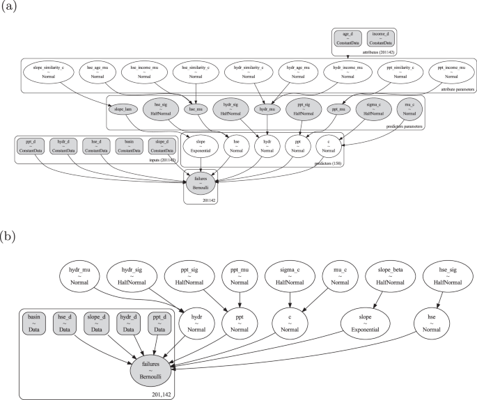
a Represent hierarchical Bayesian model, and b pooled Bayesian model, all tasked in predicting the probability of wastewater system’s failure.

Full size image

Note that a GLM, using logistic regression under maximum likelihood was not considered because it is equivalent to our pooled Bayesian model specified with non-informative priors on the parameters (Eq. (9)).

Training, evaluation, and robustness analysis

First, we constructed a dataframe that relates individual OWTS with the predictors and group-level attributes. Since precipitation, hydraulic conductivity, and topographic slope data are in raster format, we select the corresponding pixel value that is closest to each OWTS point. For median housing value, age, and income, we associate the county-level value to all OWTS that belong there. Thereafter, we perform a z-normalization for the predictors and group-level attributes to ensure a consistent scaling for each variable. In addition, we reclassify systems with status “Addition” and “New” to 0 (non-failing) and “Repair” to 1 (failing). However, the proportion of these two classes is imbalanced, with 28% representing failing and 72% non-failing systems. To prevent the model from over-fitting to the latter, we randomly pick the same number of failing to non-failing systems at each model run. Thereafter, we divide the balanced data into training and testing set using a 80:20 split, and evaluate the model’s performance across five separate runs. The hyperparameters of our ML models are tuned using k-fold cross-validation (k = 3)³⁶. Since our label is a binary variable, we use percentage accuracy as our metric to evaluate performance. Subsequently, we perform an ablation study on our pooled and hierarchical Bayesian models to evaluate how different predictor affects prediction accuracy. During ablation, we also check for multicollinearity or dependence between predictors using the Variance Inflation Factor (VIF). The higher the VIF value is, the more related the variables are, which can potentially undermine the significance of individual factors. For each predictor, its corresponding VIF value is computed as in Eq. (16), where VIF_i < 2 generally indicates low correlation of variable i relative to others³⁷. ({R}_{i}^{2}) denotes the coefficient of determination when regressing the independent variable, i, on the remaining ones.

In addition to accuracy and confusion matrices, we consider an out-of-sample goodness-of-fit (GoF) test using the Widely-applicable Information Criterion (WAIC)³⁸. This test analyzes how sensitive or uncertain a prediction is to variation in predictors and parameters. In general, the GoF tests in a Bayesian setting have a general form as defined in Eq. (17):

Where fit measures how well the learned parameters can reconstruct the target variable from a set of predictors, and penalty captures the variation of estimate to individual parameter. For this work, we consider Eqs. (18) and (19) to compute the fit and penalty, respectively.

Where, s denotes the total number of data points, n the number of predictors, and (hat{theta }) the fitted parameter indexed by j. Overall, a model with lower GoF value is more robust, and hence better for out-of-sample inferences.

After ensuring that our Bayesian models are sufficiently well-posed (e.g., stationarity and convergence tests of Markov Chain Monte Carlo parameter sampling; see Supplementary Fig. 6 for details), we compare the standard deviation of parameters in the hierarchical model before (prior) and after (posterior) fitting, as shown in Supplementary Figs. 7 and 8. The relatively low posterior variance across predictors compared to the prior variance (e.g., the parameter variance for extreme precipitation is 10 in the prior and 0.3 in the posterior distribution) suggests the importance of data over prior specification in favoring a narrow range of parameter values, resulting in a more precise data-driven prediction.

However, a Bayesian model with low posterior variance may suggest overfitting and lack robustness in predicting an out-of-sample dataset. Such model is of little value for our out-of-state inference task where ground truth data for finetuning is not currently available. To evaluate this possibility, we conduct a GoF using WAIC defined in Eqs. (17)–(19). Essentially, we aim to determine how well a model performs given variations and perturbations in both the dataset and parameter space. If a model overfits the training data, its performance in this test will be poor. Supplementary Fig. 10 plots WAIC against the relative standard error (SE), which is a vital diagnostic for measuring the uncertainty of WAIC computation and, in turn, the relative stability of a model in predicting out-of-sample cases and its sensitivity to parameter perturbation. As depicted in Supplementary Fig. 10a, hierarchical Bayesian models (represented by the blue dots) exhibit lower WAIC (better fit) and lower relative SE (more robust to out-of-sample prediction and less sensitive to parameter variation) than their pooled counterparts. When we examine the different configurations of our hierarchical Bayesian models in Supplementary Fig. 10b, we find that those trained on all predictors (labeled as “Full”) are more robust than any single-predictor model. A robust model that performs well to out-of-sample tests is crucial to ensure a reliable inference to out-of-distribution predictors, as is the case for our subsequent inference in the broader Southeastern US where the availability of ground-truth data is extremely sparse at best.

Mapping risk estimate and its uncertainty

We use our fitted hierarchical Bayesian model to infer the probability of OWTS failure in Georgia and its neighboring states which constitute the Southeastern US. The inferred states include Georgia, Florida, Alabama, Tennessee, South Carolina, North Carolina, Kentucky, Virginia, West Virginia, Arkansas, Louisiana, and Mississippi. Similar pre-processing steps are performed during inference, including z-normalization of the predictors and group-level attributes. Then, the median values of annual precipitation maxima, topographic slope, soil hydraulic conductivity, median housing, age, and income are computed in each county. Thereafter, we estimate (hat{theta }) by drawing 100 posterior samples conditioned on county-level attributes. Essentially, this step ensures that counties with similar group-level attributes exhibit similar risk level. Using a Bernoulli distribution that has been parameterized by (hat{theta }), we run the model 500 times to generate our risk estimate and its uncertainty as captured by the sample mean and standard deviation, respectively. Our uncertainty estimate is finally normalized with the risk estimate.

Cluster and correlation analyses

We perform two sets of correlation analyses to quantify the associative strength between each predictor and our risk estimate (and its uncertainty) using Pearson’s correlation coefficient. The first set includes a pairwise analysis on the county-level predictors, while the second one on the cluster level, using z-scores that are computed from the local Gi^*(d) statistic (local Getis-Ord statistic, Eq. (20))³⁹:

x_j denotes the value of each variable (i.e., precipitation, soil hydraulic conductivity, topographic slope, median housing value, risk estimate, and risk uncertainty) at county j and w_i,j the spatial weight between counties i and j. The spatial weights are defined using the Queen’s contiguity criteria, where an adjacent county that shares common border has a spatial weight of 1, or 0 otherwise. W_i is the sum of all weights w_i,j, and (scriptstyle{s}=sqrt{frac{1}{nmathop{sum }nolimits_{j = 1}^{n}{x}_{j}^{2}-{bar{x}}^{2}}}). Figure 6 illustrates clusters for each of the predictor (precipitation, soil hydraulic conductivity, topographic slope, and median housing value) and the risk outputs (mean estimate and uncertainty). For each county, the Getis-Ord statistic quantifies the z and p values. The z-score describes the type and intensity of spatial clustering; positive number indicates clusters of high-valued regions (hotspots), and negative number clusters of low values (coldspots). The higher the absolute z-score is, the more intense the clustering becomes. The p-value, on the other hand, describes statistical significance of the z-score estimate. In this study, we categorize counties with p-values greater than 0.05 as non-significant and assign a z-score of 0 (no spatial clustering).

In conclusion, future work can incorporate the notion of vulnerability to assist stakeholders in making a more informed decision. Also, including future projections of precipitation, housing values, and demographic factors can make risk maps more valuable to assist scenario-based decision-making in an uncertain future. Overall, our work aims to support the monitoring and understanding of decentralized wastewater systems by estimating their risk of failure and their associated uncertainty. With a rapidly aging OWTS infrastructure in the country, identifying key risk factors can help allocate finite resources more efficiently and effectively. Ultimately, improving wastewater infrastructure through well-informed policy not only enhances public health but also promotes equitable access to clean water as basic human rights.