Insights into defect cluster formation in non-stoichiometric wustite (Fe1−xO) at elevated temperatures: accurate force field from deep learning

Wüstite has been extensively studied in fields such as iron metallurgy, catalysis, nanoparticles, and industrial waste recycling^1,2. It is characterized as an oxide with a NaCl-type structure, featuring a high proportion of iron vacancies and a portion of iron ions occupying interstitial sites. This class of oxides also includes NiO and CoO. They can be represented by the general formula M_1−xO, where the increase in non-stoichiometry x follows the order^3,4:

The defect concentration in Fe_1−xO is extremely high, and the interactions of these defects within the solid phase are very complex. Crystallographic determinations indicate that these defects are not randomly distributed within the lattice. Various models of iron vacancy and interstitial atom clusters are proposed. Using the Kröger and Vink notation⁵, the formula for this oxide can be written as:

In this notation, Fe²⁺ and Fe³⁺ at octahedral sites are represented as ({{Fe}_{Fe}}^{circ},) and ({{Fe}_{Fe}},), respectively, while Fe³⁺ at tetrahedral (interstitial) sites is represented as ({{{Fe}}_{i}}^{{circ}, {circ}, {circ} },). Iron vacancies are denoted as ({{V}_{{Fe}}}^{q({prime} )},), which can have charges corresponding to q = 2 or q = 1, or be neutral with q = 0. Electrical neutrality can be achieved through the transition of electrons in the conduction band or through interactions with holes in the valence band. The recently evaluated band gap of wüstite is approximately 1.0 eV (at 25 °C), indicating that at high temperatures and under certain oxygen partial pressures, a significant number of electrons in the conduction band and/or holes in the valence band can be expected⁶.

The high non-stoichiometry of Fe_1−xO results in strong interactions between defects, leading to the formation of defect complexes and larger defect aggregates. Initially, Roth⁷, based on neutron diffraction studies of wüstite, proposed defect complexes composed of iron vacancies and iron interstitials, labeled as ‘2VFeFei’. Koch and Cohen⁸, through single-crystal X-ray diffraction studies of Fe_0.902O, introduced the concept of a basic cluster and proposed the [13:4] cluster (Fig. 1c), where 13 represents the total number of vacancies and 4 represents the number of tetrahedral interstitials. Lebreton and Hobbs⁹ modeled and calculated the electron diffraction pattern of [12:4] defect clusters (Fig. 1c). The results were consistent with experimental observations, leading them to conclude that the [12:4] defect clusters are responsible for the non-stoichiometry of Fe_0.872O. Catlow and Fender¹⁰ used the HADES1 code to study in detail the relative stability of defect clusters in wüstite. They suggested that [4:1] clusters could form [6:2] or [8:3] clusters by sharing faces and found that larger aggregates, see Fig. 1a, b. They discovered that the [6:2] and [8:3] clusters are more favorably bound than larger aggregates, such as the Koch-Cohen [13:4] cluster and the [16:5] spin-type cluster. Tomlinson¹¹ extended this work, identifying the Lebreton–Hobbs [12:4] cluster also as the preferred large defect aggregate. However, the parameters derived by Catlow and Fender do not accurately predict the relevant structures¹².

a The typical [4:1] defect as the basic unit; b clusters formed along the 〈100〉 direction; c clusters formed along the 〈110〉 direction; d clusters formed along the 〈111〉 direction. Squares represent Fe²⁺ vacancies, and gray spheres represent Fe³⁺ interstitials.

Full size image

The simulation techniques used to determine the aforementioned defect models (and in the present study) heavily rely on interatomic potential parameters. Anderson and colleagues¹³ applied an approximate quantum mechanical molecular orbital method and predicted the relatively high stability of clusters with a zincblende-type structure, including edge-sharing [10:4], [13:5], and [16:7] clusters. However, Anderson’s method did not account for lattice relaxation effects, which undoubtedly affect the relative stability of the clusters. Press and Ellis¹⁴, using more rigorous quantum mechanical calculations based on local density approximation, found that repulsion is reduced when [4:1] units are connected along 〈110〉 and 〈111〉 directions, see Fig. 1c, d. Nevertheless, the Koch–Cohen [13:4] cluster was still predicted to be relatively unstable. The complex situation of defect disorder in FeO has led to a series of conflicting reports. Also, due to computational limitations, the above methods can only consider the relaxation response of lattice ions around defect clusters and cannot extend the models to larger atomic systems.

Molecular dynamics (MD) simulations serve as effective tools for gaining insight into the phenomena occurring during the evolution of lattice defects in wustite. While reactive force fields (ReaxFFs) have been applied in areas such as pure liquid iron, nanoparticle systems, and surface oxidation, recent research¹⁵ has found that MD simulation results for iron oxide exhibit significant dispersion due to the iron oxide being beyond the training objectives of any existing force field, rendering it inaccurate for describing FeO systems. The latest advancements in deep learning for many-body potential energy representations bring new hope for addressing the challenges of accuracy and efficiency in molecular simulations. Deep potential molecular dynamics (DeepMD) utilizes density functional theory (DFT) calculations as datasets and is capable of accurately describing large-scale atomic systems^16,17,18,19.

In this study, potential parameters suitable for the FeO solid-phase system were developed using deep learning methods. The parameters were validated against experimental and density functional theory (DFT) results, highlighting their advantages over the currently commonly used ReaxFF molecular dynamics. Based on this, the formation pathways of typical defect clusters in wüstite were analyzed, identifying the low energy barriers and structural stability of the Koch–Cohen defect cluster.

Energies and atomic forces

Ten systems for AIMD calculations were first constructed to generate the raw data, including the atomic coordinates, atomic energies, and forces, as the initial training data set for DP training. The ten systems include (1) bulk phase of FeO crystal with the equilibrium lattice constants (labeled as Bulk_100) and scaled lattice constant with a scale factor of 0.95 and 1.05 (labeled as Bulk_095 and Bulk_105, respectively); (2) vacancy structures with a single vacancy and double vacancy, as shown in Fig. 2a–d. A system with one Fe atom removed and one O atom removed was labeled as Vac_1Fe and Vac_1O, respectively. A system with two Fe atoms removed and two O atoms removed was labeled as Vac_2Fe and Vac_2O; (3) Surface structures with (001), (110), and (111) orientations, which were labeled as Sur_001, Sur_110, and Sur_111, respectively, as shown in Fig. 2e–g.

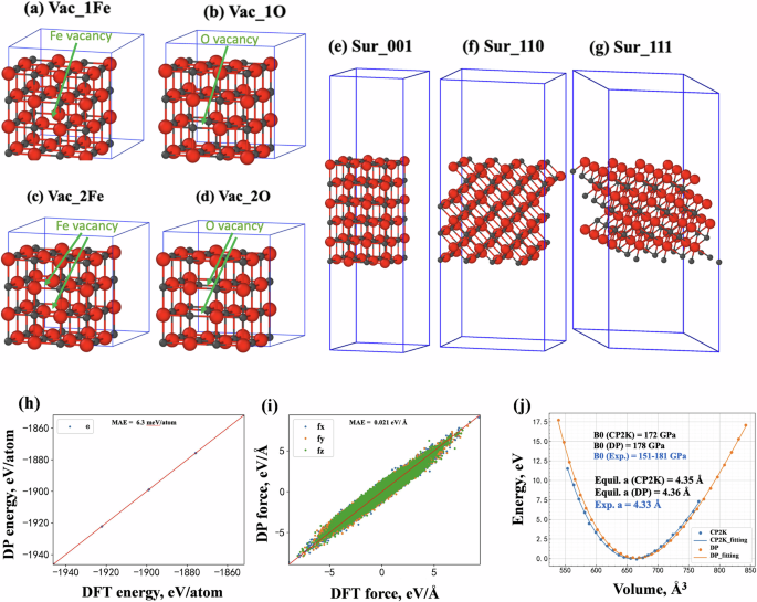
a–d represent vacancy structure with one Fe atom removed, one O atom removed, two Fe atoms removed, and two O atoms removed, respectively. e–g represents a surface structure with the orientation of (001), (110), and (111), respectively. The gray and red colors represent the Fe and O atoms, respectively; Comparisons of h energies, i forces, and j the final equation of states for FeO calculated by DeepMD and DFT, the Birch–Murnaghan⁷³ method was used to fit the EOS curves. The solid red lines represent y = x, indicating that the results predicted by DeepMD match perfectly with DFT.

Full size image

In this work, a total of 24 iterations were performed to obtain the final accurate datasets (10,268 configurations) and DP function, with 400,000 steps of deep learning in each iteration, as shown in Table S1. The general principle to make the order of the iterations is to make the datasets become more and more complex with the increasing iteration steps. Figure 2h–j compares the energies and atomic forces predicted by DFT and DP for all the structures in the final training database. It indicates a close agreement between DP predictions and DFT results with a mean absolute error (MAE) of 6.3 meV/atom for energy and 0.021 eV/Å for force. The equation of state for FeO was also calculated using DP, and the results are shown in Fig. 2j. The final obtained equilibrium lattice of FeO is 4.36 Å, which is very close to the DFT result (4.35 Å) and the experimental result (4.33 Å)^20,21. The calculated bulk modulus using DP is 178 Gpa, which is also in agreement with the DFT result (172 GPa) and is in the range of experimental bulk modulus (151–181 GPa)^20,21. The agreement of energy, force, lattice constant, and bulk modulus between DFT and DP demonstrated that the DP potential had been well-trained for the FeO system.

A comparison of the formation energies for single and double vacancies of oxygen and iron atoms in wüstite, using DeepMD potential parameters and DFT calculations, is presented in Fig. S1. The results indicate that the formation energy of oxygen vacancies is in good agreement with the DFT calculation results, with an error margin below 1%, demonstrating the efficacy of the deep learning potential parameters in handling oxygen vacancies. The formation energy of a single Fe vacancy (DFT: 6.58 eV, DeepMD: 4.97 eV) is consistent with existing studies (DFT: 3.75–6.99 eV²², experimental value: 5.61 eV²³). There is still relatively high error in the single vacancy calculations, indicating limitations of the DeepMD potential in accurately describing the magnetic properties and charge states of iron-containing systems. Specifically, the training set used for DeepMD development did not explicitly incorporate different charge states of Fe vacancies, which are known to significantly influence defect formation energies. Addressing this limitation by including charge state information in the training data represents a potential direction for future optimization^24,25. However, the error in the formation energy of double vacancies is significantly reduced (from 24.4% to 6.8%), making the computational accuracy for large-scale systems with multiple vacancies still acceptable.

Non-stoichiometry of wustite (Fe_1−xO)

The currently used ReaxFF potential parameters for Fe–O systems are based on the work of various researchers focusing on Fe–O cluster systems^26,27. Comparing Fig. 3a, b, under the DeepMD potential parameters, the Fe–O system retained the NaCl-type lattice structure of wüstite, whereas the ReaxFF potential parameters failed to maintain this structure. The Fe_1−xO structures computed using six typical ReaxFF potential parameters^{26,27,28,29,30,31} are shown in Fig. S2, none of which retain the wüstite lattice structure. The RDF results calculated using six existing ReaxFF potential parameters are compared in Fig. 3c. Under the DeepMD potential parameters, the atomic distances between Fe and O are concentrated around 2.2 Å, which is consistent with the experimentally obtained lattice parameters of Fe–O. In contrast, the distances calculated using ReaxFF potential parameters are significantly lower than the experimental values.

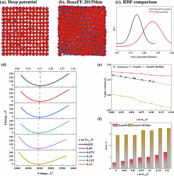
a Fe_1−x O structure after structural relaxation under the DP potential; b Fe_1−xO structure after structural relaxation under the ReaxFF potential; c RDF results comparison between DP and ReaxFF potentials; d EOS curves for structures with different numbers of iron vacancies; e Variation of lattice constants with iron vacancies; (Comparison between DP potential, ReaxFF potential, and experimental values); f lattice constant calculation errors relative to experimental values.

Full size image

To elucidate the nature of non-stoichiometry in wustite (Fe_1−xO), the a forementioned 14 × 14 × 14 FeO system was used, where varying proportions (2.5%, 5%, 7.5%, 10%, 12.5%, 15%) of iron atoms were randomly deleted. Each configuration was then systematically scaled (scaling factor from 0.95 to 1.05 with a step size of 0.01) and subjected to static energy calculations to obtain the equation of state (EOS) for each configuration, as shown in Fig. 3d. The lowest point of each curve represents the stable state of that configuration, thus providing the relationship between the wustite lattice structure and x. As the x value increases, the minimum point of the EOS curve shifts to the left, indicating that the volume of the stable state configuration of Fe_1−xO gradually decreases. The comparison between the DeepMD and ReaxFF potentials is illustrated in Fig. 3e. The red curve shows that as the number of Fe vacancies in wustite increases, the lattice constant gradually decreases, maintaining good consistency with experimental values and with minimal error (Fig. 3f). This is the first time that large-scale dynamic simulation of iron oxide lattice structures has been achieved at the atomic scale.

Defect cluster structure of Wustite (Fe_1−xO)

When an iron vacancy occurs in FeO, it results in six oxygen atoms becoming unsaturated. This unsaturation attracts the surrounding octahedral iron atoms, which can easily migrate towards the unsaturated oxygen atoms, forming interstitial tetrahedral iron atoms that remain stable, as shown in Fig. 4a (highlighting the interstitial iron atoms). Figure 4b shows the evolution of interstitial iron atoms over time, from rapid formation to gradual stabilization. As the value of x increases, the maximum number of interstitial iron atoms also increases significantly.

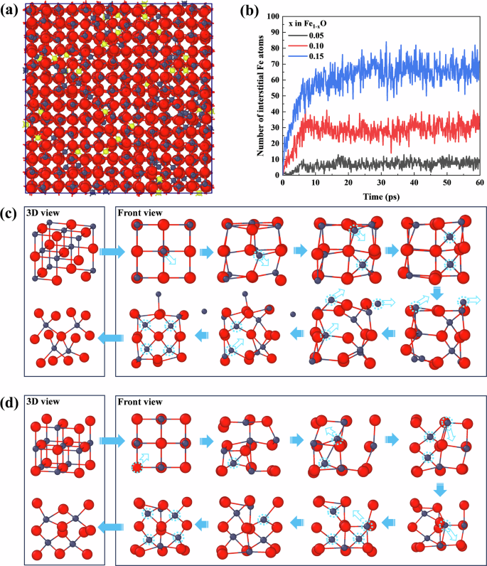
a interstitial Fe atoms in the FeO structure (highlighted in yellow); b temporal evolution of interstitial Fe atoms during structural optimization; c formation process of the typical [10:4] defect; d formation process of the typical [13:4] (Koch–Cohen) defect. Fe atoms are displayed in gray, and O atoms are displayed in red.

Full size image

Defect clusters are concentrated along the 〈110〉 direction. The formation process of a typical [10:4] defect cluster along the 〈110〉 direction is shown in Fig. 4c. Initially, an octahedral iron atom moves towards an iron vacancy, creating an interstitial iron atom and leaving behind a new iron vacancy. This triggers a chain reaction where neighboring octahedral iron atoms further migrate to the newly formed vacancies, creating new interstitial iron atoms that stabilize. The system reaches a locally stable state; however, as new iron atoms migrate outward, the equilibrium is disrupted. This causes additional octahedral iron atoms to transform into interstitial tetrahedral iron atoms, ultimately forming stable typical [10:4] defect clusters. The formation process of the most common Koch–Cohen defect clusters is shown in Fig. 4d. Initially, two tetrahedral interstitial iron atoms are generated along the 〈110〉 direction. Unlike the [10:4] defect, which further forms octahedral interstitial iron atoms around an oxygen atom, the Koch-Cohen defect cluster [13:4] forms around one of the iron vacancy defects, with surrounding iron atoms migrating one by one.

The diffusion coefficient of iron atoms in wüstite (−7 cm² s⁻¹ < log₁₀D < −5 cm² s⁻¹, Fig. 5a, b) matches well with experimental results^32,33. Self-diffusion primarily occurs via a vacancy-driven mechanism. At a given temperature, the self-diffusion coefficient D_Fe increases with the increase in x (Fig. 5c). As the temperature T increases, the dissociation of clusters leads to an increase in the number of free vacancies, thereby increasing the self-diffusion coefficient (Fig. 5d). This is consistent with the in-situ diffusion studies by Rickert and Weppner³⁴, as well as the isotope studies by Desmarescaux and Lacombe³⁵. Figure S3 presents the Arrhenius plot for D_s, showing an activation energy of 22.74 kJ mol⁻¹.

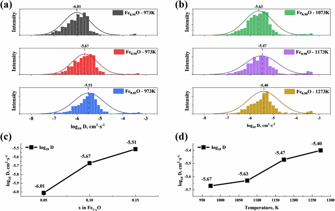
a diffusion coefficient of iron atoms in Fe_1−xO at different x values; b diffusion coefficient of iron atoms in Fe_0.9O at different temperatures; c relationship between diffusion coefficient and x in Fe_1−xO; d relationship between diffusion coefficient and temperature.

Full size image

Using the obtained potential parameters, the NEB method was employed to calculate the formation pathways of different defect clusters in wustite along three crystallographic directions, as shown in Fig. 6. The formation of defect clusters in all three directions begins with the migration of an iron atom after the first iron vacancy appears, creating an interstitial iron atom, which forms the basic unit of the [4:1] defect cluster. This process, with an energy barrier of 0.036 eV, leads to a stable intermediate. Along the 〈100〉 direction (Fig. 6a), successive stacking of [4:1] defects results in the formation of [6:2], [8:3], and [10:4] defect clusters, with energy barriers of 1.42 eV, 0.93 eV, and 0.86 eV, respectively. The rate-limiting step in this direction is the formation of the [6:2] cluster structure. In contrast, in the 〈110〉 direction (Fig. 6b), the formation of the second [4:1] unit is relatively easy, requiring only a 0.13 eV energy barrier to form the [7:2] configuration. From this point, the cluster can develop in two directions: either centered around an oxygen atom, overcoming energy barriers of 0.32 eV and 0.66 eV to form the [10:4] defect cluster, or centered around an iron vacancy, overcoming energy barriers of 0.48 eV and 0.56 eV to form the [13:4] (Koch–Cohen) defect cluster. In both pathways, the rate-limiting step is the formation of the fourth [4:1] defect cluster, with the [13:4] (Koch–Cohen) cluster being relatively easier to form. Along the 〈111〉 direction (Fig. 6c), the formation of the second [4:1] defect is the rate-limiting step, with a high energy barrier of 1.82 eV. Subsequent energy barriers of 0.49 eV and 1.53 eV lead to the formation of the [13:4] configuration.

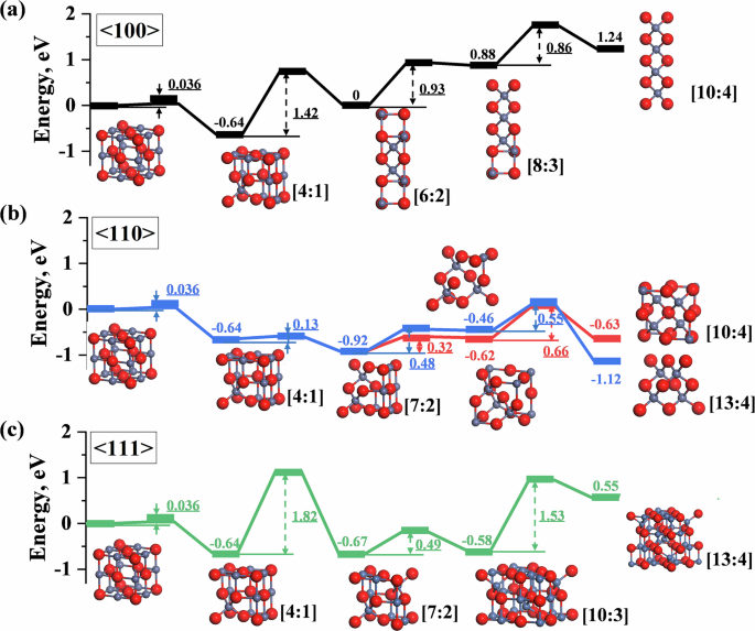
a 〈100〉; b 〈110〉; c 〈111〉. Fe atoms are displayed in gray, and O atoms are displayed in red.

Full size image

When using the original configuration as a reference, the relative energy of the defect clusters increases progressively as the stacking along the 〈100〉 direction proceeds. The energy of the [8:3] and [10:4] defect clusters exceeds 0, indicating that the stability of the structure diminishes as more than three [4:1] units are stacked, making the formation process more challenging than the reverse process. In the 〈110〉 direction, however, all defect clusters have energies below 0, and except for the stacking of the third [4:1] defect, the energy decreases progressively. The [13:4] (Koch–Cohen) cluster exhibits the lowest relative energy, confirming that the stacking process in this direction is favorable in terms of structural stability. In the 〈111〉 direction, the [10:3] configuration has the lowest relative energy, and further stacking of [4:1] defects is no longer advantageous. The NEB calculation results for the formation pathway of the typical [13:4] (Koch–Cohen) cluster using DFT are presented in Fig. S4. The DeepMD potential shows consistency with DFT in both results and trends; however, discrepancies arise due to the higher convergence precision of DFT. A comparison of computational time further highlights the significant advantage of the DeepMD potential in terms of efficiency.

Through the training of deep learning potential parameters, this study has, for the first time, achieved large-scale dynamic simulations of iron oxide lattice structures at the atomic scale, yielding highly accurate results. By comparing experimental data, ReaxFF potential parameters, and DFT calculations, the DeepMD potential successfully modeled the lattice structure, diffusion behavior, and defect structures of non-stoichiometric wüstite. As the number of iron vacancies in wüstite increased, the lattice size gradually decreased (Fig. 3). This reduction is attributed to the increasing number of interstitial iron atoms (Fig. 4), which leads to the formation of numerous defect clusters. According to the calculation results shown in Fig. S1, although the formation energy of the first iron vacancy is high, the formation energy for a new iron vacancy near an existing one is significantly reduced, indicating a tendency for iron vacancies to cluster and form locally stable structures. Additionally, as the number of iron vacancies increases, the diffusivity of iron atoms also gradually increases (Fig. 5), facilitating the formation of stable defect cluster structures.

By comparing the formation pathways of defect clusters in different directions (Fig. 6), it was found that the [13:4] (Koch–Cohen) defect cluster along the 〈110〉 direction has the lowest process energy and configuration energy, making it the most stable defect cluster configuration. In contrast, stacking more than three tetrahedral iron atoms along the 〈100〉 and 〈111〉 directions does not favor structural stability. This is because the four [4:1] units along the 〈110〉 direction support each other, leading to saturated dangling bonds and resulting in a locally stable structure.

Although the atomic-scale simulation of iron oxide defects achieved in this study demonstrates stable and accurate results, the current deep learning approach still faces several challenges. First, the deep learning model used in this work does not incorporate charge information as part of the input data, relying solely on the mapping relationship between atomic coordinates and energy. This limitation may account for the model’s reduced ability to describe oxygen vacancy defects accurately (Fig. S1). Integrating charge information into deep learning-based molecular dynamics simulations is a promising direction for future improvement. Additionally, as the dataset for this study was generated using AIMD simulations, the preparation of the initial dataset requires significant computational resources and may result in insufficient sampling of rare events. In future research, enhanced sampling methods, such as metadynamics^36,37, could be employed to complement the potential energy surface sampling for rare events.

DFT calculations

Density functional theory (DFT) with the Gaussian Plane Wave (GPW) method, as implemented in the QUICKSTEP module of the CP2K code³⁸, was used to calculate the spin-polarized electronic. To avoid the explicit consideration for the core electrons, the scalar-relativistic norm-conserving pseudopotentials of Goedecker, Teter, and Hutter (GTH)^39,40 were applied. A linear combination of contracted Gaussian-type orbitals using MOLOPT basis sets optimized for the corresponding GTH pseudopotentials⁴¹ was used to describe the wave functions of the valence electrons. The exchange and correlation energy were calculated using the exchange-correlation functional of Perdew, Burke, and Ernzerhof (PBE)^42,43. For configurations containing defects, a homogeneous neutralizing background charge^38,44 is applied to address charge imbalance due to defect formation under periodic boundary conditions.

Conventional DFT is known to underestimate the Coulomb repulsion between the localized 3d-electrons of Fe^45,46. The DFT + U method was applied to obtain a more accurate description of these states^47,48. In this semi-empirical approach, an additional potential is applied to the 3d-states of iron. The evolution of total energy and relative DFT + U energy vs lattice constant with U values ranging from 0 to 2.0 eV is shown in Fig. S5a, b, respectively. All the U values produce a similar equation of state curves as the quantum espresso (QE) results²⁰. The physically acceptable values of U must result in positive DFT + U energy⁴⁶, limiting the range of U < 1.5 eV. The Hubbard parameter is known to influence the electronic spectrum through the on-site Coulomb repulsion profoundly. The unoccupied Fe states were shifted to higher energies, while the occupied Fe states were unchanged. The value of the band gap increased monotonically with the increscent Hubbard parameter (Fig. S5c). In the conventional DFT (U = 0 eV), there is no noticeable band gap for Fe (red line in Fig. S5c). The experimentally measured value and theoretical value of the band gap for wustite ranged differently (0.5–2.4 eV)^20,21,49 due to the different experimental conditions and the non-stoichiometric character of wustite. To ensure a positive DFT + U energy with an acceptable band gap, U = 1.4 eV, which produces an energy gap at about 0.55 eV, was selected for further ab initial calculations. For simplicity, the antiferromagnetic ordering was set along the [001] direction as both [001] direction and [111] direction produce similar lattice structure²⁰. The simulations were performed in a 2 × 2 × 2 supercell of FeO crystal after convergence tests showing that both 2 × 2 × 2, 3 × 3 × 3 and 4 × 4 × 4 produce the same results. The energy bands obtained in the simulation are in good agreement with experimental data, as detailed in Supplemental Fig. S6.

An auxiliary double-ζ valence polarized (DZVP) basis set⁴¹ of plane waves was employed to expand the electronic density using an electronic density cutoff of 600 Ry and a relative electronic density cutoff of 80 Ry. The selection of these two cutoff energies is based on the results shown in Supplemental Fig. S7, where one cutoff energy was fixed while the evolution of energy was calculated as the other cutoff was varied. Considering the computational resource requirements, the test results in Fig. S7 validate that the combination of 600 Ry and 80 Ry ensures sufficient accuracy. The calculations of vacancy formation energies were performed for relaxed structures, with energy convergence accuracy set to 1 × 10⁻¹⁴, and the corresponding convergence curves are provided in Supplemental Fig. S8.

The Néel temperature of wustite is around 200 K⁵⁰, above which FeO transitions from an antiferromagnetic state to a paramagnetic state. Considering that the non-stoichiometry nature and the environment significantly influence the Néel temperature⁵¹, and our tests showed that the lattice structure of FeO is not accurate if antiferromagnetic characteristics are not set in CP2K, the antiferromagnetic setting is kept in all the ab initio calculations in CP2K. Further study is required regarding the influence of high temperature and defects on the magnetic properties of wustite. Possible strategies include incorporating temperature-dependent potentials to account for thermal effects and improving defect models by incorporating charge states at elevated temperatures. Enhanced computational methods, such as Monte Carlo simulations or metadynamics, could also be used to improve the modeling of magnetic behavior under high-temperature conditions.

With the optimized DFT parameters, the final equation of the state of FeO crystal is obtained, as shown in Fig. 2d. The equilibrium lattice constant is 4.35 Å, which is in close agreement with the experimental value (4.33 Å^20,21). The fitted bulk modulus with Birch–Monaghan method⁵² is in the range of 167–172 GPa, which is also in good agreement with the experimental range (151–181 GPa)^20,21. The agreement between the calculated properties (lattice constant, bulk modulus, band gap) and the experimental results validated the robustness of the DFT parameters adopted.

DeepMD potential

The deep neural network (DNN) was constructed following the method recently proposed by Zhang et al.^16,17,18,19. Data generated from DFT and AIMD simulations, including energy, force, virial, box dimensions, and atom types, are transferred from the Data Generator to the DeePMD-kit Train/Test module to enable training^18,19. The DeePMD-kit framework has been widely validated for its reliability and accuracy in modeling complex interactions across diverse material systems^53,54,55,56, though challenges in incorporating charge information remain an area for future improvement. A potential optimization strategy has been reported in Tao’s recent works^24,25, which developed machine-learned force fields for different charge states of iodide interstitials and vacancies in CsPbI₃. Schematic of the DeePMD-kit architecture and the workflow are shown in Fig. S9¹⁹. In this scheme, the potential energy E of each atomic configuration is obtained by summing the “atomic energies” with the following equation:

where E_i is determined by the local environment of atom i within a smooth cutoff radius Rc. E_i is constructed in two steps. First, a set of symmetry-preserving descriptors is constructed for each atom with the Deep Potential Smooth Edition (DeepPot-SE) constructed from all atomic configuration information (both angular and radial)¹⁷. Next, the information of descriptors is given as input for a DNN, which returns E_i as the output. The additive form of E naturally preserves the extensive character of the potential energy. With this method, the DNN potential has been validated to reproduce interatomic forces and energies predicted by DFT accurately for a wide range of systems^{57,58,59,60,61,62,63,64,65,66}.

Concurrent training

Constructing accurate and generalized deep potential functions, which determine the relationship between the potential energy E_i of one atom and the environment of its neighboring atoms, is achieved using an accurate initial data set and an active learning strategy. AIMD simulations were performed with the above ten systems in the NVT ensemble (constant number of atoms, volume, and temperature) at 73 K, 573 K, 1073 K, and 1573 K using the Noseé–Hoover thermostat⁶⁷ and run for 750–1500 steps with 0.5 fs time step. The data were collected every ten AIMD steps, and finally, 2655 training samples were obtained as the initial datasets, and 660 untrained samples were kept for validation. It was thought that the final converged DP model was not sensitive to the exact construction of the initial training database⁶⁸.

The second step is to improve the generality and accuracy of the DP model by an active learning strategy of adequate sampling on the potential energy surface (PES) coupled with an accurate DFT computation. This is achieved by Deep Potential GENerator (DP-gen)^57,68 software for iteration, where each complete iteration consists of DP training (by DeePMD-kit)^18,19, DP molecular dynamics exploration (by LAMMPS)⁶⁹, and DFT recalculation (by CP2K)³⁸. The detailed iteration process is as follows: four DP models are learned using the same training set. The embedding and fitting nets contained three layers with the nodes [25, 50, 100] and [240, 240, 240], respectively. The smoothing parameters r_cs and r_c values were 0.5 Å and 8 Å, respectively. The weight coefficients of energy in the loss functions increase from 0.02 to 1, while the weight coefficients of force in the loss function decrease from 2000 to 1 during the training process. Second, the exact MD sampling of the structures is performed using the four DP models, and the structures requiring DFT recalculation are screened by calculation of the model force error between the models:

where f_i denotes the force on atom i. In the present study, ({delta }_{f}^{min }) and ({delta }_{f}^{max }) are set to 0.08 and 0.28 eV/Å. Configurations with a relative deviation less than ({delta }_{f}^{min }) are labeled as “accurate”. Configurations with a relation deviation in the range of ({delta }_{f}^{min }) − ({delta }_{f}^{max }) are labeled as “candidates” for the training data sets. Configurations with a relation deviation larger than ({delta }_{f}^{max }) are excluded, as a relatively poor model drives the exploration in this region.

Large-scale simulation

Large-scale simulations were conducted on a 14 × 14 × 14 FeO system containing 2744 atoms. The non-stoichiometric wüstite (Fe_1−xO) structure was modeled by randomly deleting Fe atoms at a proportion of x. With a timestep of 0.1 fs, molecular dynamics simulations were performed using DeepMD and ReaxFF potential parameters at 300 K for 20,000 steps to achieve structural relaxation. The temperature was then gradually increased to 800 K over 20,000 steps and maintained at that temperature for another 20,000 steps, with the NPT ensemble applied throughout the process. The minimum energy path for the defect cluster formation process was calculated using the NEB method^70,71,72, implemented in LAMMPS.

Calculation of diffusion coefficients

The diffusion coefficient D for Fe atom was calculated using the mean squared displacement (MSD) method. The MSD was computed from the trajectories of 1000 randomly selected atoms over a time interval of 0.4 ps. Specifically, for each selected atom, the displacement Δr(t) was calculated, and the MSD was obtained by averaging the squared displacements over all time steps:

where ({r}_{i}(t)) is the position of the i-th atom at time t, and N is the number of atoms in the selected group. The diffusion coefficient D was determined from the long-time limit of the MSD using the Einstein relation:

where t is the time, and the factor of 6 accounts for the three-dimensional nature of the system. To ensure accurate results, the diffusion coefficient was calculated over a specific time window, defined by the start and end times based on the trajectory data. The calculated diffusion coefficients for each atom were then plotted to show their distribution.