Integrative whole slide image and spatial transcriptomics analysis with QuST and QuPath

Introduction
Spatial analysis, a critical component of pathology, has greatly enhanced our understanding of complex biological processes. Traditional pathology, which involves scrutinizing tissue slides with high-power microscopy, is labor-intensive. However, the advent of digital image analysis (DIA) and machine learning (ML) technologies has broadened the scope of artificial intelligence (AI) in this field. Over the past few years, a slew of deep learning (DL) based whole slide image (WSI) analysis tools such as QuPath1, TIA Toolbox2, MONAI3, SlideFlow4, PHARAOH5, WSInfer6 have been introduced.
One of the significant hurdles in DL-based WSI analysis is the creation of training patterns. Hematoxylin & eosin (H&E), the standard tissue staining technique, provides structural information but rarely offers direct biological evidence like gene expressions and transcription factors. As a result, the success of DL-based WSI analysis hinges largely on the expertise of those conducting manual annotation tasks on the WSI H&E images.
On the other hand, spatial transcriptomics (ST) has seen significant advancements as it enables the visualization and analysis of histological sections with gene expression features. ST provides valuable spatial context to molecular data, making it vital for studying complex biological processes, such as cell-cell interactions. ST also presents a unique opportunity to address the challenges of DL-based WSI analysis, as subcellular ST technologies are already available. However, merging these two powerful modalities has been challenging due to differences in data formats and analyzing methods.
Numerous studies have delved into the application of tools for the analysis of ST in WSI. For example, Wood et al. examined the use of QuPath for image analysis, paired with GeoMx ST, to investigate gene expression variability in colorectal cancer and liver metastases7. Tippani et al. also have highlighted the necessity of bridging high-resolution images for spatially resolved transcriptomics data, and concluded the missing capabilities of QuPath for supporting preprocessing of the multichannel fluorescent images. Despite certain constraints, QuPath’s significant functionalities in image analysis have been widely recognized. Nonetheless, these studies mainly use QuPath for initial analysis, with detailed ST analysis done using other tools.
While providers of ST technologies have developed various platforms for visually examining and researching biological insights from given samples, such as Loupe Browser (https://www.10xgenomics.com/support/software/loupe-browser/latest), Xenium Explorer (https://www.10xgenomics.com/support/software/xenium-explorer/latest), and AtoMx Spatial Informatics Platform (https://nanostring.com/products/atomx-spatial-informatics-platform/atomx-sip-overview/), these tools have not fully exploited the functionalities of DIA, resulting in ineffective integration of existing DIA tools and platforms into ST research. To address this gap, we present QuST, a QuPath extension that offers a comprehensive platform for integrating and analyzing WSI and ST data. QuST is designed to enable more in-depth spatial-omics analysis, including cell-cell interactions, cell spatial profiling, and visualization. Furthermore, QuST’s implementation of Deep Learning (DL)-based cell categorization and region segmentation methods could facilitate image annotation based on biological evidence.
Methods
QuST is designed to seamlessly integrate WSI and ST analysis with QuPath, enhancing its capabilities with tools specifically tailored for spatial biology. The extension supports the visualization of spatial gene expression data within the context of histopathological images, enabling users to explore the molecular landscape of tissues at an unprecedented resolution (see Fig. 1). Below, we will introduce some analyzing tools and use cases available in QuST.

a Users begin by importing ST data into QuPath using QuST. This step may require additional spatial alignment data which can be generated via FIJI (see Fig. 2), if the user is working on Xenium dataset (see text). b Once the ST data is successfully loaded, users can perform analysis and visualization via QuPath and QuST. c Given the biological evidence provided by ST, users can generate the training set for image based cell classification and region segmentation based on H&E. Finally, the result generated using the DL module can be further analyzed using the functions described in b.
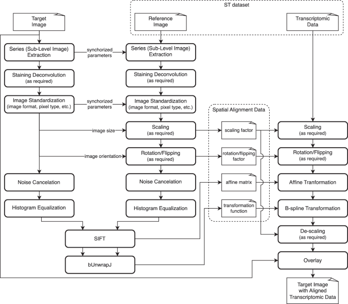
The procedure generates SIFT affine matrix and B-spline transformation function, mapping the coordinations in the reference image (e.g., DAPI) to the given target image (e.g., H&E).
Integrative WSI and ST analysis at single-cell level
QuST is being developed with a focus on single-cell level analysis. It has the capability to load single-cell level ST data formats, including those from 10x Genomics Xenium and NanoString CosMx. Furthermore, it can also load 10x Genomics Visium datasets for whole-slide, full-spectrum ST analysis.
A significant challenge in single-cell level ST analysis lies in aligning ST data with WSI, primarily due to the involvement of different image modalities. For instance, in Xenium and CosMx, cell localization relies on DAPI staining, while WSIs can be H&E staining. This necessitates multiple rounds of sample preparation and scanning to acquire multiple staining of the samples. Consequently, loading ST data requires extra steps for aligning the ST data with the provided WSI. To address this issue, we took inspiration from the guidelines provided by 10x Genomics (https://www.10xgenomics.com/analysis-guides/he-to-xenium-dapi-image-registration-with-fiji), and proposed a method that aligns the coordinates of ST data to the reference image, as illustrated in Fig. 2.
To test the proposed approach, in the experiment, we first performed a cell detection algorithm, e.g., StarDist8, Cellpose9, etc. Then, for experimental purpose, we loaded transcriptomic data with and without including image registration information, separately. The results are shown in Fig. 3, and the statistical evaluation of cell displacement between the H&E image and transcriptomic data is shown in Fig. 4. In the experiment, 723,384 cells were detected from H&E images. Without using image registration, 122,288 cells were missing. The root causes include: 1) different quality control approaches for the two data modalities; and 2) the location information obtained from the transcriptomic data did not match the cells detected on the given H&E images. With image registration, this number dropped to 99,405, representing an 18.71% improvement. In addition, it can be observed that the deformation looks much relevant to the grid-like artifacts10 resulting from stitching the DAPI images (see Fig. 3e, f). As a result, integrating the proposed ST and WSI registration can mitigate the noises generated from data acquisition.
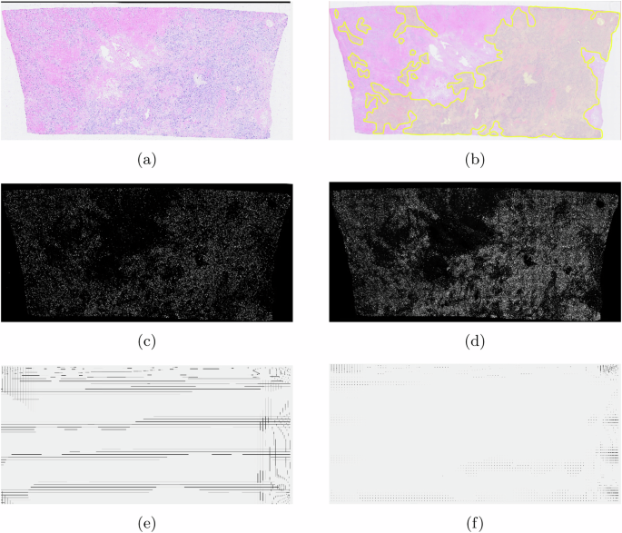
a–b The target image; c The Hematoxylin channel of the target image; d DAPI asthe reference image; e–f The deformation for image registration.
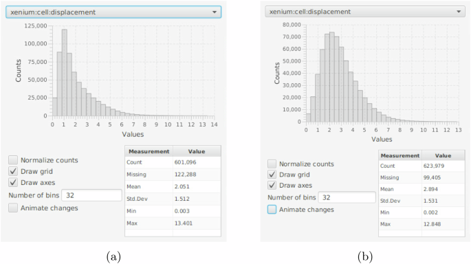
a The result generated without using image registration. b The result generated using image registration.
For performing whole-slide, full-spectrum ST analysis using 10x Genomics Visium datasets, QuST requires the corresponding affine matrix, generated manually via the Visium Image Alignment function in the Loupe Browser (see https://www.10xgenomics.com/support/software/space-ranger/latest/analysis/inputs/image-fiducial-alignment). In addition, in the work of HEST-1k11, an automatic fiducial detection using the YOLOv8 model12 was introduced, which enables alignment inference for full-spectrum ST and WSI interactive analysis using Visium datasets.
Cellular spatial profiling
Cell spatial profiling plays a critical role in spatial-omics analysis. In QuST, cell spatial profiling provides the foundation of all other spatial related computing. First, the Delaunay clustering is required in order to obtain the neighboring cell connectivity. Next, the edge distance of each chosen cells is computed. As a result, the position of each cell in the cluster is obtained and can be used for the following analyzing tasks. The detailed algorithm is shown in Algorithm 1.
The results shown in Fig. 5 represent insights from cellular spatial analysis. The heat map indicates the boundary distance of individual cells, e.g., the distance from a cancer epithelial cell to the boundary of the corresponding tumor boundary. Based on the heat map, one can explore the differential gene expression patterns between the intratumoral tumor cells and the tumor cells present in the immune-invasive region, which are located on the surface of the tumor.
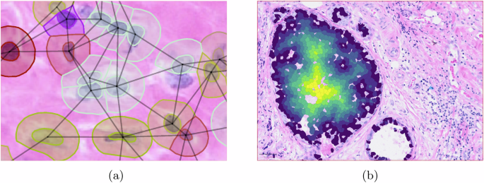
a Neighboring cell connectivity based on Delaunay clustering. Various single cell analyses available in QuST are based on the neighboring cell connectivity. b QuST’s cellular spatial profiling generates a heat map indicating the distance to boundary of a specific cell type, e.g., tumor-epithelial cells to the corresponding tumor boundary.
A use case of QuST is spatial profiling for tumor micro-environment (TME). The TME encompasses the surrounding cellular and non-cellular components that interact with cancer cells. It plays a crucial role in tumor growth, progression, and response to therapy. By understanding the complex interactions between cancer cells, immune cells, stromal cells, and the extracellular matrix, researchers can identify potential targets for therapeutic intervention. Given the rich information provided by a ST dataset, the functions that QuST can provide are of paramount importance for TME study.
Algorithm 1
Cell spatial profiling based on Delaunay clustering
1: definition
2: (C=left{{c}_{1},{c}_{2},cdots right}): all chosen cells
3: (T=left{{t}_{1},{t}_{2},cdots right}): all cell types
4: (din {{mathbb{Z}}}_{ > 0}): a threshold of edge distance defining the neighborhood of a cell
5: (kin left[mathrm{0,1}right]): a threshold for determining is c locating at the boundary of a cluster
6: ({rm{EdgeDist}}left(c,c^{prime} right)in {{mathbb{Z}}}_{ > 0}): edge distance between (c) and (c^{prime})
7: ({rm{CellType}}left(cright)in T): function for obtaining cell type of (c)
8: ({e}_{c}in {{mathbb{Z}}}_{ge 0}): the computed edge distance to the boundary of clusters, (forall cin C)
9: procedure ({rm{CellSpatialProfiling}}left(tin T:{rm{a; chosen; cell; type}}right))
10: ({e}_{c}leftarrow 0,forall cin C)
11: for each (cin C) where ({rm{CellType}}left(cright)=t), do
12: ({N}_{c}leftarrow left{{c}^{{prime} }|{rm{EdgeDist}}left(c,{c}^{{prime} }right)le {d},{bf{and}},{c}^{{prime} }ne c,forall c^{prime} in Cright}) ⊳ all neighbors of ({c})
13: ({O}_{c}leftarrow left{{c}^{{prime} }|{text{CellType}}left({c}^{{prime} }right),ne, t,forall c^{prime} in {N}_{c}right}) ⊳ all other types in neighbors of c
14: ({e}_{c}leftarrow 1,{bf{if}}frac{left|{O}_{c}right|}{left|{N}_{c}right|}ge k) ⊳ initialize ec the distance to the cluster boundary
15: ({i}1) ⊳ i: distance indicator
16: repeat
17: for each (cin C) where (text{CellType}left(cright)=t), do
18: ({N}_{c}leftarrow left{{c}^{{prime} }|{rm{EdgeDist}}left(c,{c}^{{prime} }right)le {d},{bf{and}},{c}^{{prime} }ne c,forall c^{prime} in Cright}) ⊳ all neighbors of c
19: ({O}_{c}leftarrow left{{c}^{{prime} }|text{CellType}left({c}^{{prime} }right),ne, t,forall c^{prime} in {N}_{c}right}) ⊳ all other types in neighbors of c
20: ({e}_{c}leftarrow i+1,{bf{if}}frac{left|{O}_{c}right|}{left|{N}_{c}right|}le k,{bf{and}},exists {c}^{{prime} }in {N}_{c},{e}_{{c}^{{prime} }}=i)
21: (ileftarrow i+1)
22: until (forall cin C,{e}_{c}) are obtained
return ({e}_{c},forall cin C)
Cellular neighborhood analysis
Living tissues are composed of various cellular communities that coexist in complex spatial structures. Clusters of cells, each specialized for particular tissues, function together in advanced functional units to uphold and manage organ functions. Thus, the analysis of spatial context is critical for a thorough understanding of tissue biology. Schapiro et al. proposed HistoCAT13, highlighted the potential of studying the cellular neighbors using multiplex immunohistochemistry (mIHC) imaging. In addition, Ruitenberg et al. explored the analysis of cellular neighbors in spatial omics, yielding new biological insights14. Inspired by their works, we introduced Cellular Neighborhood Analysis (CNA) (see Algorithm 2).
Algorithm 2
Cellular neighborhood analysis
1: definition
2: (C=left{{c}_{1},{c}_{2},cdots right}): all chosen cells
3: (T=left{{t}_{1},{t}_{2},cdots right}): all cell types
4: (din {{mathbb{Z}}}_{ > 0}): a threshold of edge distance defining the neighborhood of a cell
5: ({rm{EdgeDist}}left(c,c^{prime} right)in {{mathbb{Z}}}_{ > 0}): edge distance between (c) and (c^{prime})
6: ({rm{CellType}}left(cright)in T): function for obtaining cell type of (c)
7: ({h}_{c,t}in left[mathrm{0,1}right]): the probability that (t) exists in the neighborhood of (c)
8: procedure CellularNeighborhoodAnalysis
9: ({h}_{c,t}leftarrow 0,forall cin C,forall tin T)
10: for each (cin C), do
11: ({N}_{c}leftarrow left{{c}^{{prime} }|{rm{EdgeDist}}left(c,{c}^{{prime} }right)le {d},{bf{and}},{c}^{{prime} },ne, c,forall c^{prime} in Cright}) ⊳ all neighbors of c
12: for each (c^{prime} in {N}_{c}), do
13: (t^{prime} leftarrow {rm{CellType}}left(c^{prime} right))
14: ({h}_{c,t^{prime} }leftarrow {h}_{c,t^{prime} }+1)
15: ({h}_{c,t^{prime} }leftarrow {h}_{c,{t}^{{prime} }}/left|{N}_{c}right|,forall t^{prime} in T)
return ({h}_{c,t},forall cin C,forall tin T)
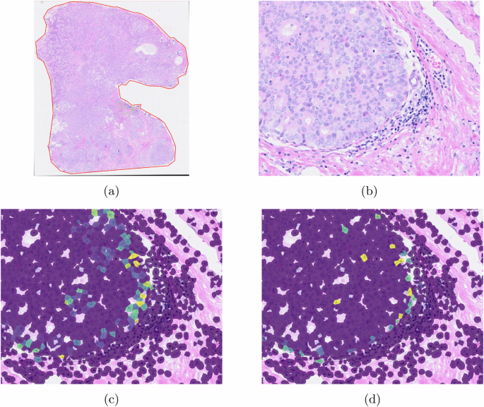
An outcome is depicted in Fig. 6. In the experiment, we initially emphasized the epithelial and tumor cells. We then carried out CNA and used a heat map to display the count of lymphocytes that could be identified in the vicinity of a cell. By overlaying the tumor regions and the CNA results, one can determine the likelihood of a tumor cell having at least one lymphocyte in its immediate surroundings.
a The given whole slide image. b The chosen ROI for the experiment. c Epithelial and tumor cells are highlighted as reference. d The heat map indicates the number of lymphocytes that can be found in the neighbors of a cell.
Cell-cell interaction analysis
ST is a powerful tool for understanding cell-cell interactions (CCIs) within tissues. By mapping gene expression patterns and spatial organization, researchers gain insights into how cells communicate and influence each other. This knowledge has implications for drug development, disease research, and personalized medicine.
QuST uses the datasets provided by CellTalkDB15, which is a manual curated database that provides a comprehensive collection of ligand-receptor (LR) pairs in both humans and mice. The database includes 3398 human LR pairs and 2033 mouse LR pairs, which were obtained through a combination of text mining, manual verification of known protein-protein interactions using the STRING database, and literature-supported evidence for each pair.
QuST uses the results of cellular spatial profiling to compute CCI, incorporating crucial information about cell neighborhoods within specific regions of interest. When analyzing a cell of receptors, QuST takes into account all ligand cells situated within a designated neighboring distance, determined using Delaunay clustering, for the computation of the corresponding CCI. The algorithm presented in Algorithms 2 provide detailed explanations of how QuST calculates the LR product. Our future work includes incorporating implementations for more advanced methods15.
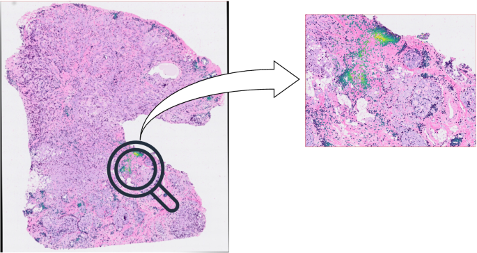
Figure 7 shows a result of CCI, focusing on CEACAM6-EGFR CCI analysis. As CCI analysis offers an additional layer of investigation by generating a heat map that illustrates the intensity of CCI for a specific ligand-receptor pair. The generated heat map provides a quantitative measure of the strength and significance of communication among a cluster of cells.
a The given WSI. b The ROI shows a region of tumor and lymphocyte aggregation. c CCI ligand (CEACAM6) expression. d CCI receptor (EGFR) expression.
Algorithm 3
Ligand/Receptor expression computing for CCI based on LR product
1: definition
2: (C=left{{c}_{1},{c}_{2},cdots right}): all chosen cells
3: (Q=left{{left(l,rright)}_{1},{left(l,rright)}_{2},cdots right}): all chosen ligand-receptor pairs
4: (din {{mathbb{Z}}}_{ > 0}): a threshold of edge distance defining the neighborhood of a cell
5: ({rm{EdgeDist}}left(c,c^{prime} right)in {{mathbb{Z}}}_{ > 0}): edge distance between (c) and (c^{prime})
6: (text{LigExpr}left(c,lright)in {{mathbb{R}}}_{ge 0}): ligand (l) expression of (c)
7: (text{RecExpr}left(c,rright)in {{mathbb{R}}}_{ge 0}): receptor (r) expression of (c)
8: ({v}_{c,left(l,rright),l}in {{mathbb{R}}}_{ge 0}): ligand expression of the given (c) and (left(l,rright))
9: ({v}_{c,left(l,rright),r}in {{mathbb{R}}}_{ge 0}): receptor expression of the given (c) and (left(l,rright))
10: procedure ({rm{CCIProfiling}})
11: ({v}_{c,left(l,rright),l}leftarrow 0,forall cin C,forall left(l,rright)in Q)
12: ({v}_{c,left(l,rright),r}leftarrow 0,forall cin C,forall left(l,rright)in Q)
13: for each (cin C), do
14: ({N}_{c}leftarrow left{{c}^{{prime} }|{rm{EdgeDist}}left(c,{c}^{{prime} }right)le {d},{bf{and}},{c}^{{prime} }ne c,forall c^{prime} in Cright}) ⊳ all neighbors of c
15: for each (left(l,rright)in Q), do
16: for each (c^{prime} {in N}_{c}), do
17: ({v}_{c,left(l,rright),l}leftarrow {v}_{c,left(l,rright),l}+text{LigExpr}left(c,lright)times text{RecExpr}left(c^{prime} ,rright))
18: ({v}_{c,left(l,rright),r}leftarrow {v}_{c,left(l,rright),r}+text{RecExpr}left(c,rright)times text{LigExpr}left(c^{prime} ,lright))
19: ({v}_{c,left(l,rright),l}leftarrow {v}_{c,left(l,rright),l}/left|{N}_{c}right|)
20: ({v}_{c,left(l,rright),r}leftarrow {v}_{c,left(l,rright),r}/left|{N}_{c}right|)
return ({v}_{c,left(l,rright),l},{v}_{c,left(l,rright),r},forall cin C,forall left(l,rright)in Q)
Cell clustering analysis
Recent research has highlighted the profound relationship between the functioning of various biological processes, such as cell-cell interactions, and the local densities and positions of cells within cellular monolayers and stratified epithelia. In an attempt to delve deeper into this relationship, Küchenhoff et al. introduced DBSCAN-CellX, a density-based clustering algorithm16 to study cell densities and positions within cellular monolayers and stratified epithelia, crucial for understanding various biological processes. This algorithm extends the DBSCAN method17 to analyze cell localization and tissue physiology. For example, it has been noted that Tertiary Lymphoid Structures (TLSes) are associated with a favorable cancer prognosis18. Furthermore, a technique for identifying TLS and evaluating their density on H&E-stained digital slides of lung cancer was proposed19.
To facilitate cell clustering analysis, we integrated DBSCAN-CellX into QuST. Given the classes of the cells, QuST is able to compute local densities and positions of cells accordingly. The results are shown as the measurements in the detection table. Hence, the results can also be visually investigated and exported using the native QuPath functions of measurement maps.
The result is shown in Fig. 8, indicating that clusters of lymphocytes (50+) were identified from the given sample. This integration allows researchers to utilize DBSCAN-CellX directly for quantitatively analyzing lymphocyte clusters, potentially identifying imaging biomarkers that correlate with disease prognosis.
(left) Clusters of lymphocytes (50+) were identified from this example. (right) The color annotated on a selected cell indicates the “edge degree” of the cell, which refers to the distance to the edge of the corresponding lymphocyte cluster.
Pseudo spot generation based on single cell ST data
While sub-cellular ST technologies exist, they often have limitations in terms of the range of the genome they can cover. Consequently, lower-resolution technologies capable of analyzing the entire genome continue to be widely used. As a result, there is a requirement to generate data for evaluating gene expression deconvolution approaches.
QuST provides an opportunity to evaluate the spatial single cell deconvolution methods by mimicking the Visium datasets (see Fig. 9). For example, Huang et al. proposed an approach of ST auto-encoder and deconvolution method, largely utilizing the integration of a scalable deep generative model for predicting gene expression at cellular or nuclei level based on H&E imaging and in situ RNA capturing, thus allowing a better understanding of the tissue micro-environment20.
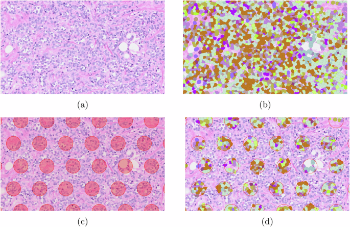
a The chosen ROI. b Single cell data. c Generated pseudo spots. d Pseudo spots containing single cell data.
DL-based image classification and segmentation with QuPath
QuST primary utility lies in utilizing transcriptomic data as the biological basis for training deep learning-based object categorization and region segmentation for H&E images. To service this purpose, QuST features functions for extracting single-cell H&E images for cell classification, as well as WSI patches for region segmentation. The QuPath annotation and detection measurement tables can be exported as files, serving as image label data for DL model training. Consequently, QuST significantly reduces the workload for users training their models for WSI analysis.
QuST includes a DL capability based on PyTorch21 to perform image classification, which aids in cell categorization and region segmentation tasks. To initiate the training procedure, two inputs are required. Firstly, an image set in a folder generated using the aforementioned image sampling approach. Secondly, the detection/annotation measurement table, which can be directly generated from QuPath measurement functions. QuST offers a wide range of neural networks, including resnet22, vgg23, densenet24, and various variations of modern vision transformers (ViT)25.
Object classification
In the experiment, we first acquired H&E image patches for each detected object (e.g., a cell). Next, we used the genotype information provided by the chosen datasets, and train the DL model for object classification. In this experiment, we used ViT. A confusion matrix, shown in Fig. 10, was computed based on 10-fold cross-validation. Some examples of single-cell genotype classification based on H&E are shown in Fig. 11. In our experiment, as shown in the confusion matrix, cell types 1 and 10 can be better predicted based on single-cell H&E images, while type 4 has a poor prediction result. This result revealed that certain cell types are more readily distinguishable in H&E staining, such as lymphocytes, blood cells, etc., while others are not. Furthermore, differentiating B-cells from T-cells based on H&E staining is recognized as a particularly challenging task.
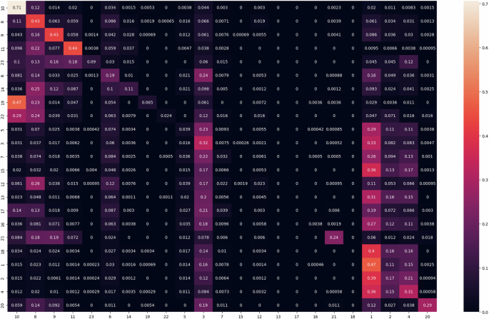
The result showed that cell types 1 and 10 can be better predicted using H&E images.
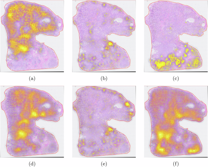
a–c The ground truth samples. d–f The predicted outcomes.
Region segmentation
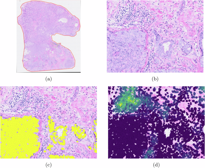
In the experiment, we used manual annotation as shown in Fig. 12a. The chosen model was resnet50. The testing target is shown in Fig. 12b. Based on 10-fold cross-validation, we obtained the confusion matrix shown in Fig. 13.
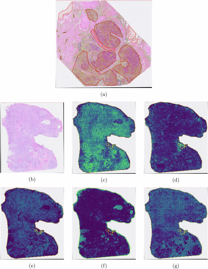
a The H&E image as the training data used in this experiment. b The testing image. c Tumor regions. d Immune regions. e Tumor regions. f Adipose regions. g Necrosis regions.
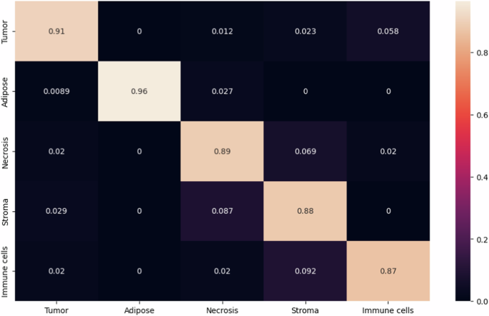
The result showed a good performance for region segmentation for tumor, adipose, necrosis, stroma and immune regions on H&E images.
In addition, QuST also provides region segmentation with arbitrary tile size (aka. resolution). The higher the resolution, the longer the processing time. Figure 14 shows an example of various resolutions for region segmentation.
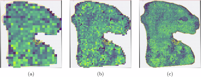
The color of heat map of each tile indicates the probability that the tile belongs to a tumor region. Various tile sizes are presented. a 400μm. b 200μm. c 50μm.
Responses