Label-free live cell recognition and tracking for biological discoveries and translational applications

Label-free live cell microscope-based analysis refers to single timepoint or longitudinal monitoring of cell population behaviours in the absence of phototoxicity and labelling reagents, and is typically accomplished with the aid of computer vision algorithms due to the tedious nature of manual techniques. Within this context, it is imperative for biologists to have a solid understanding of computer vision algorithm principles and methodologies in order to capitalise on this approach’s potential to contribute towards basic and translational biomedical research. Such knowledge is crucial for biologists to make sound biological inferences and communicate with computer vision scientists when algorithms fall short of expectations. Likewise, it is equally vital for computer vision scientists to be intimately familiar with the objectives of biologists, so that their algorithm development efforts are specifically targeted for their end users’ needs.

To facilitate a clear and in-depth discussion, it is imperative for both algorithm developers (computer vision scientists) and end-users (biologists and biomedical researchers) to clarify the definition of ‘cell recognition’, which may be conflated with various Computer Science definitions associated with different levels of task complexity. For a given input (Fig. 1a), images may be categorised as to whether cells are present or absent, which is termed ‘classification’ (Fig. 1b), or alternatively localised via different methods (Fig. 1c–f). These latter localisation methods may involve using bounding boxes to delineate the approximate coordinates of individual cells, which is called ‘object detection and localisation’ (Fig. 1c), binary masks to distinguish background and foreground/cell regions, which is known as ‘semantic segmentation’ (Fig. 1d), individual masks to distinguish each cell, which is termed ‘instance segmentation’ (Fig. 1e), and individual masks that distinguish each cell as well as their cell type, which is delineated as ‘panoptic segmentation’ (Fig. 1f). In this review, ‘cell recognition’ is interchangeably used with ‘instance segmentation’, whereby distinct regions or masks (i.e. pixels) are allocated to each individual cell.

a A Zernike’s qualitative phase contrast microscope (ZPCM) image is used as input. b At the simplest level, the input image can be subjected to classification, which ascertains the presence or absence of cells in a given image. c At a low level of complexity, objects can be detected and localised via bounding boxes, which can also distinguish different categories such as cell types. d At a medium level of complexity, pixel-wise classification or sematic segmentation may be performed to distinguish foreground and background. e At a high level of complexity, individual objects (cells) may be distinguished via instance segmentation. f At a very high level of complexity, individual objects belonging to different categories (e.g. different cell types) may be distinguished via panoptic segmentation. Purple bounding boxes/outlines and green outlines in (c) and (f) enclose segmented cells. Black and white in (d) indicate background and foreground/cell regions, respectively. Different coloured masks indicate instance segmented cells.

Full size image

In terms of addressing the broad range of scientific questions and applications sought by biologists and biomedical researchers, label-free live cell instance segmentation and tracking is a highly versatile technique. In a typical analysis, individual cells and their resulting cell trajectories are recognised in single images and image sequences, respectively. This enables a single microscope sample to generate multiple metrics or readouts regardless of whether the sample is comprised of a single timepoint or multiple timepoints (Fig. 2). Single timepoint measurements may include various cell morphological readouts including its relative intensity, size, shape, perimeter, texture features, etc. that indicate the cell’s status such as whether the cell has undergone differentiation, mitosis, apoptosis, quiescence, senescence, etc. (Fig. 2). Multiple timepoint measurements may include not only the metrics derivable from single timepoint measurements but also additional readouts such as migration speed and genealogy/lineage information (Fig. 2). In addition, biological readouts can also be computed at the level of individual cells as well as for a given cell population. Individual biological metrics may include cell morphology, proliferation, differentiation, quiescence, migration, etc. whereas population-level metrics include cell heterogeneity, cell lineage tree, confluency, etc. (Table 1). Due to the label-free nature of these methodologies and use of transmitted white light (i.e. there is little-to-no phototoxicity and no labelling reagents to impact experimental outcomes), the readouts are representative of cells in their unperturbed or ‘natural’ state, offering valuable biological insights and potential inroads for translational applications. Hypothetically, these attributes may be useful, for example, in identifying unproductive stem cell donors for biomanufacturing (Fig. 2). In a notable example of biological discovery, Gilbert et al. performed long-term tracking of individual muscle stem cells grown in hydrogel microwells to show that substrate stiffness can affect muscle stem cell differentiation and survival¹. As a demonstration of proof-of-concept for potential translational application, Ker et al. monitored time-dependent changes in myoblast confluency to demonstrate use of cell segmentation algorithms for cell biomanufacturing². As such, label-free approaches enable researchers to attain individual or multiple snapshots of cell populations at the resolution of single cells that can discover new cellular behaviours and aid development of therapeutics for regenerative medicine.

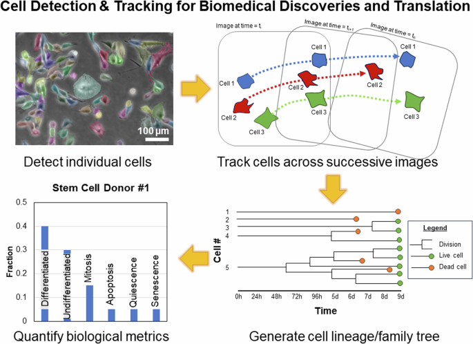
Instance segmentation and tracking of cells across successive images enable cost-effective, real-time monitoring of cells to generate complex biological metrics to quantify cell behaviours at the level of single individual cells and whole cell populations. Different biological metrics may be used to define productive and unproductive donors to efficiently streamline a biomanufacturing process.

Full size image

Given the wide breadth of basic and translational applications that may utilise label-free live cell analysis, deployment of this technology is expected to have significant impact on biomedical research productivity and translational applications. For example, there were an estimated 2,737,640 biomedical-related research articles published during 2017 to 2019³ and commercial applications for label free cell analysis has a projected market size of USD 829.71 million dollars by 2028⁴. In this regard, label-free live cell analysis can increase productivity by reducing or eliminating labour-intensive and time-consuming steps often performed in biomedical research. Notably, many regenerative medicine therapeutics involve cell-based strategies that require biomedical scientists to culture stem/progenitor cells for lengthy durations followed by labour-intensive staining to assess levels of differentiation. In work by Waisman et al., a convolutional neural network classifier was reported to detect induced pluripotent cell differentiation in unstained cells within 1 h of switching to induction media⁵. Also, Sasaki et al. reported that, with a LASSO regression model, cellular morphologies can be used to predict mesenchymal stem cell differentiation into multiple lineages including osteocytes, adipocytes, and chondrocytes⁶. Possessing such capabilities to predict cell behaviour is important, particularly in the context of expanding cells for biomanufacturing, where multi-timepoint readings such as cell confluency must be closely monitored to maintain stemness and avoid undesired cell differentiation². In addition to predicting cell differentiation, label-free cell instance segmentation and tracking can contribute towards semi-automated, high-throughput disease diagnosis⁷ and drug discoveries⁸. Together, label-free live cell analysis can improve biomedical research productivity.

Label-free live cell instance segmentation and tracking can be accomplished by numerous sensing modalities including but not limited to brightfield microscopy, Zernike’s qualitative phase contrast microscopy (ZPCM), differential interference contrast (DIC)/Nomarski microscopy, electrical cell impedance sensing (ECIS), quantitative phase imaging (QPI) methods, and imaging flow cytometry. In the following section, common modalities for label-free live cell instance segmentation and tracking are briefly introduced in terms of their working principle, advantages, and disadvantages followed by an assessment on their preferential use.

Brightfield imaging is one of the simplest and cheapest forms of optical microscopy and can be found in most biological laboratories. In brief, this technique visualises a sample by passing illumination light through the sample with contrast generated due to the absorption of light by denser areas of the specimen^9,10,11,12. This imaging technique is compatible with standard tissue culture vessels and its spatial and temporal resolution is dependent on both microscope objectives and camera hardware acquisition speed, respectively (Table 2)^9,10,11,12. However, the semi-transparent nature of cells makes morphological details challenging to be easily visualised with high clarity (Table 2)^9,10,11,12. Since brightfield microscopy is amenable to optical sectioning, there have been recent efforts to improve upon the technique by using optical sectioning to generate 3D brightfield image stacks¹³. Subsequently, standard digital filters can be applied to reconstruct these 3D image stack and allow for accurate visualisation of optically thin objects¹³.

ZPCM is a highly ubiquitous and low-cost microscope imaging modality that visualises cells with high contrast. Relative to brightfield microscopy, the fundamental basis behind this technique is the addition of a condenser annulus and phase plate that transform differences in the optical path length (after light has passed through a phase object such as a cell) into intensity changes (Table 2)^{9,11,12,14,15}. Since optical path length differences are related to an object’s thickness and refractive index, high contrast can be generated for subcellular structures (Table 2)^{9,11,12,14,15}. This allows for imaging of birefringent or dichroic specimens such as muscle tissue while maintaining its compatibility with standard tissue culture vessels (Table 2)^{9,11,12,14,15}. Although ZPCM images may invariably contain artefacts such as undesired halos that obscure cellular details^{9,11,12,14,15}, such features may be capitalised upon for cell instance segmentation^16,17. Similar to brightfield microscopy, the spatial and temporal resolution of this technique is dependent on both microscope objectives and camera hardware acquisition speed, respectively, with good optical sectioning capability for relatively thin specimens (Table 2)^{9,11,12,14,15}.

DIC/Nomarski microscopy is an optical technique that introduces contrast to specimens with a pseudo 3D effect. This microscope imaging modality is highly popular but not nearly as ubiquitous as brightfield or ZPCM due to a slightly more stringent requirement for strain-free objectives and additional costly optical elements such as Nomarski or Wollaston prisms^9,12,14. The operating principle behind DIC microscopy is the use of polarised light to convert the phase delays that result after passing through a biological specimen into intensity changes for generating contrast^9,12,14. Unlike typical ZPCM imaging, this contrasting effect is created locally in adjacent structures that possess different refractive indices (i.e. optical path length gradient for DIC/Nomarksi microscopy versus optical path length magnitude for ZPCM), producing the aforementioned pseudo 3D image with reduced halo artefacts^9,12,14. Although these local optical path length gradients can be utilised for cell instance segmentation¹⁸, this pseudo 3D topography can often be confusing to novice microscopists. Also, this imaging technique is typically not compatible with dichroic or birefringent specimens including standard tissue culture vessels due to optical disturbances caused by differential absorption of polarised light’s ordinary and extraordinary wave components^9,12,14. Similar to both brightfield and ZPCM, the spatial and temporal resolution of this technique is dependent on both microscope objectives and camera hardware acquisition speed, respectively, with an optical sectioning capability that is generally better than ZPCM for relatively thick specimens (Table 2)^9,12,14.

ECIS is an alternative cell sensing approach that is less ubiquitous than the afore-mentioned microscope modalities due to its higher cost for specialised, high-end electronic hardware. ECIS measures electrical impedance distributions across cell bodies by injecting low-frequency electrical current that is suitable for sensing dynamic changes such as cell proliferation, apoptosis, differentiation, etc. (Table 2)^19,20,21. There are no cell images or optical sectioning capability associated with this methodology and the requirement to inject low-frequency electrical current for cell sensing requires use of specialised culture vessels containing sterile and disposable electrode arrays (Table 2)^19,20,21. As a result, there is poor lateral (xy) spatial resolution due to technical challenges in packing numerous electrodes together for distinguishing individual cells within confluent cultures (Table 2)^19,20,21. However, ECIS has high axial (Z) spatial resolution on the order of 1 nm¹⁹ as well as high temporal resolution for monitoring time-dependent cell behavioural changes (Table 2)^19,20,21. The latter is useful for measuring fast biological events as long as readings are not confounded by noise originating from fluctuations in pH or medium composition (Table 2)^19,20,21.

Rather than a single technology, QPI techniques are a collection of methods that, similar to ZPCM, attain information (e.g. thickness and optical density) of objects being imaged via detection of phase shifts as light passes through them. A recent review by Nguyen et al. has comprehensively explained the principles and applications behind different QPI techniques which include interferometry-, digital holography-, wavefront sensing-, and phase retrieval algorithm-based methods and are not further elaborated upon here²². A distinct advantage of QPI methods over ZPCM is their quantitative nature, which generates high contrast reconstructed images of cells without artefacts such as halos (Table 2)^{22,23,24,25,26}. In addition, the quantitative nature of QPI techniques can provide physical and chemical properties of cells such as the height/topography of cells^27,28 or cell biomechanical attributes^27,29, and the concentration of biomolecules such as haemoglobin^27,30 as well as cell behaviours and dynamics such as cell growth^27,31 and transmembrane water flux^27,32. Such information can be useful to distinguish cell types and study cellular events vital for homoeostasis and pathogenesis²⁷. To keep the remarks on QPI brief, readers are referred to excellent reviews by Lee et al.²⁷, Nguyen et al.²², and Park et al.²⁵. While the lack of imaging artefacts may facilitate higher ease of annotation for cell segmentation²³, QPI methods typically require specialised, expensive and complicated setups (Table 2)²⁶, which impede its widespread adoption. Also, although the spatial resolution is dependent on QPI methodology, the need for image reconstruction typically results in poor temporal resolution, precluding its use for studying rapid biological events (Table 2)^{22,23,24,25,26}. Typically, QPI methods are compatible with standard tissue culture vessels and do not possess optical sectioning capabilities (Table 2)^{22,23,24,25,26}. However, QPI variants such as gradient light interference microscopy (GLIM) possess excellent optical sectioning capabilities for thick specimens but exhibit incompatibility with standard tissue culture vessels (Table 2)^{22,23,24,25,26}. Recent efforts have combined different techniques to overcome some of the drawbacks of QPI methods²⁶. This includes use of an inexpensive, white light wavefront sensing that only requires minor modifications to a conventional microscope to generate QPI images²⁶.

Imaging flow cytometry is an approach that combines the high throughput nature of traditional flow cytometry with high-speed imaging of individual cells. As an extension of conventional flow cytometry, both label-free (i.e. light scatter and image acquisition) and label-based (i.e. fluorescence staining of cells) measurements are used^33,34. While data acquired using non-label-free measurements may be considered outside the scope of this review, a variation of this technique known as ghost cytometry uses can be considered label-free owing to the use of in silico labelling^35,36. In brief, labelled and label-free data attained from imaging flow cytometry are used to train a machine learning-based algorithm so that it can distinguish between different cell types and cell states such as viability and differentiation^35,36. After machine learning, the imaging flow cytometer can be used in label-free mode to screen and sort cells^35,36. Potential applications include diagnostics such as leukaemia detection^33,34,35, drug discovery approaches such as cell phenotypic screening^33,34,37, and cell biomanufacturing such as enrichment of stem cell-derived progenitors^33,34,38. Ghost cytometry typically requires specialised and expensive setups found in imaging flow cytometers such as multiple lasers (for labelled measurements) and detectors that can capture biological events at high speeds, which results in high cost and impedes widespread adoption (Table 2)^33,34. Also, owing to the use of fluidics to measure suspension/dissociated cells, ghost cytometry has high throughput and single cell resolution but poor temporal resolution that precludes its use for tracking cells (Table 2)^33,34. Since the measurement is performed on dissociated cells, compatibility with standard tissue culture vessels and optical sectioning capabilities are not applicable (Table 2)^33,34.

When comparing the benefits and drawbacks for these label-free live cell imaging techniques, several key considerations emerge. These include whether a particular technique is simple, affordable, widely available, and generates high contrast information of cells to facilitate accurate cell instance segmentation. For example, while brightfield microscopy is simple, ubiquitous, and has good optical sectioning capability, the low contrast images of cells attained from this technique are a major impediment towards cell instance segmentation and tracking algorithms (Table 2). ZPCM imaging is similarly simple and ubiquitous with good optical sectioning capability for thin specimens as well as the added benefit of generating high contrast cell images despite suffering from halo artefacts (Table 2). Although other techniques such as DIC, QPI, ECIS, and ghost cytometry may be free of such halo artefacts, they typically have special requirements such as tissue culture vessels with low birefringence (i.e. DIC) or potentially expensive and cumbersome setups (i.e. ECIS, QPI, and ghost cytometry), which hinder ease of experimentation and widespread use, respectively (Table 2). Indeed, among these imaging modalities, ZPCM remains one of the most common techniques used by biologists, as indicated by the high number of search results from a simple survey of major scientific repositories for 2D microscope image datasets containing in vitro-cultured cells (Table 3). Therefore, ZPCM image data remains the most widely used for label-free imaging but at the same time, this imaging modality is greatly underutilised due to the challenges in extracting biological information.

As a technology, label-free cell instance segmentation and tracking has broad-ranging biomedical impact and significance but must overcome several obstacles to achieve widespread usage with practical performance. Indeed, instance segmentation and tracking cells without the use of staining reagents is highly challenging, for the reasons outlined below.

First, cells are highly dynamic in nature, being able to exhibit a variety of complex irregular shapes according to cell type and culture conditions³⁹. Also, they are able to grow in size, overlap (i.e. crawl over one another), and divide into daughter cells, which dramatically increases the complexity of cell instance segmentation and tracking tasks. In addition, modelling biologically relevant conditions often require cells to be cultured at high densities, which further exacerbates the difficulty for attaining precise instance segmentation and tracking due to substantial overlapping and clustering of cells. Furthermore, there is considerable variability in intensity and contrast for the same cell component⁴⁰. For example, the boundaries of a dividing cell appear progressively brighter as it detaches from the cell culture substrate to undergo mitosis in ZPCM. Similarly, the intensity signal from the boundary of a migrating cell may be perturbed by nearby cells. This lack of constant signal and contrast intensity can result in incorrect cell boundary prediction as well as mistakenly overestimating (oversegmentation) and underestimating (undersegmentation) of true cell numbers, negatively impacting biological analyses and interpretations⁴⁰. Second, gaining biological insights require sampling sufficient cell numbers for adequately powered statistical analyses⁴¹. This necessitates low magnification (e.g. 4× or 5×) cell instance segmentation and tracking, whereby each cell is only represented by several pixels. Such low information content hinders cell identification. Third, the background of images for brightfield microscopy, ZPCM, and DIC microscopy spans the typical intensity range for cells. This results in a low signal-to-noise ratio in terms of distinguishing cells from background^42,43. Unlike fluorescent images where the background pixels have zero or near-zero intensity values, this makes it particularly difficult to distinguish cells from background using intensity alone. Fourth, generating manually annotated data to develop computer vision algorithms is highly tedious and time-consuming, requiring several hundreds to thousands of man-hours as estimated by prior studies^41,44,45. Altogether, these reasons contribute towards the complexity of cell instance segmentation and tracking, which requires significant investment of resources to overcome. Therefore, there is no generic algorithm that can universally segment and track multiple cell types with great accuracy at the single cell-level.

In this review, we have introduced the concept of label-free cell instance segmentation and tracking (Introduction) and will subsequently describe a generalised pipeline for label-free live cell data generation for microscopy-based methods (i.e. brightfield microscopy, ZPCM, DIC microscopy, and QPI methods), cell annotation curation, computer vision-aided segmentation, computer vision metrics, and data mining (Workflows for Computer Vision-aided Cell Instance Segmentation, Tracking, and Biological Data Mining) followed by a review of different cell instance segmentation and tracking methods including image pre-processing, computer algorithm categorisation, performance metrics, basis and performance of instance segmentation and tracking algorithms, and considerations for future algorithmic development (Cell Instance Segmentation and Tracking Computer Vision Algorithms), as well as our outlook on label-free cell instance segmentation and tracking technology such as overcoming small datasets, development of novel algorithms, and emerging trends (Perspective). Although this review generalises the experimental pipeline as well as cell instance segmentation and tracking algorithms for microscope-based cell imaging modalities, several of the examples will utilise ZPCM on account of its preferential use in biological and biomedical research (Table 3). Also, ECIS is not elaborated upon further owing to its general inability for cell instance segmentation and tracking within confluent cultures, slightly lower usage relative to microscope-based methods, and different data modality (i.e. electrical signals instead of images) (Table 2). Therefore, this review aims to bridge the gap between biology and computer vision, recognising that not all biologists or biomedical researchers are familiar with computer vision concepts and not all computer vision scientists are familiar with microscope- and biology-associated concepts as well as the algorithm performance by end users.

To better apply computer vision-based cell instance segmentation and tracking, it is important to understand label-free live cell instance segmentation and tracking workflows including their associated hardware and software. Briefly, the process includes wet- and dry-lab research and can be divided into three sequential phases: data generation and cell annotation curation, computer vision-aided cell instance segmentation and tracking. Following completion of these workflows, biological data mining is subsequently performed.

In the first phase, label-free live cell data which can be comprised of either a single image or series of consecutive images (i.e. a time-lapse sequence)⁴¹, are acquired followed by data curation to annotate cells using a combination of hardware and software.

Numerous equipment and steps are required for acquiring label-free cell images and sequences. Generally, an inverted microscope equipped with a heated stage top incubator, humidifier, and appropriate gas cylinders and accessories for maintenance of physiological conditions, as well as on-board software for automated image acquisition are required. While such a simple setup can be homemade and customised at relatively low cost according to user requirements, commercial suppliers can provide all-in-one systems that possess additional features such as autofocus and objective heaters to prevent focus drift⁴⁶, media reservoirs and tubing for automated media changes, and accessories such as optical tables to minimise vibration and ensure levelness. In any event, these systems enable rapid, automated generation of either single- or multi-timepoint microscope images for cell instance segmentation or cell tracking, respectively.

To perform data acquisition, cells are seeded at an appropriate density in tissue culture vessels, placed on the stage top incubator to maintain cell physiological state (if image acquisition occurs over a lengthy duration), and subjected to Köhler illumination for homogenous specimen lighting before a user-defined imaging schedule is executed for automated image or video collection across different culture conditions. During data acquisition, high quality data may be collected by either utilising the microscope’s autofocus feature with use of objective heaters or maintaining a fixed focus point with an adequate period of pre-heating to ensure that cells remain focused throughout the experiment. The frequency of data acquisition is dependent on the goals of a particular experiment as well as the complexity of cell instance segmentation and tracking. Typically, higher imaging rates generate more temporal and spatial information, which is expected to improve cell instance segmentation and tracking performance, but this comes at the expense of increased dataset size and data management cost. For example, Ker et al. sought to understand the effect of various growth factors on C2C12 myoblast differentiation and used a seeding density of 2 × 10⁴ cells per 35-mm Petri dish (about 2080 cells per cm2). Due to the number of cells present over the course of the study as well as their expected migration speed, image sequences were acquired every 5 min over approximately 3.5 days, generating 49,919 images or 48 image sequences⁴¹. After acquiring the data at a suitable frequency, the image data is checked to ensure that collected image/video data are of sufficient quality (e.g. cells remained well-focused throughout the study duration), exported, and cell annotation is performed.

Acquired microscope images or image sequences need to be labelled or annotated prior to training cell instance segmentation and tracking models (in the case of supervised machine learning) or to generate reference cell annotations for assessing algorithmic performance. Although other computer vision studies have used the term ‘ground-truth’ interchangeably with reference cell annotations, it should be noted that human-curated cell annotations are not infallible and may contain errors. Therefore, the term ‘ground-truth’ is best reserved for scenarios where a particular annotation is known to be 100% correct. This includes cases where the cell image is relatively simple to annotate (i.e. few cells that are spaced far apart and not overlapping) or in the case of computer-generated cell images, where associated cell annotations are inherently known. As such, studies such as Maška et al.⁴⁷ utilise terminologies such as ‘gold standard reference corpus’ and ‘silver standard reference corpus’. In the former, reference cell annotations reflect a majority opinion from three human experts while in the latter, the reference cell annotations are computer-generated annotations ‘averaged’ from high-performing algorithms and are informed or guided by a ‘gold standard reference corpus’⁴⁷.

Typically, cells are annotated by either labelling their cell centres (known as centroids) or cell boundaries (known as masks), requiring a user either to digitally mark the centre or draw the outline of each individual cell, respectively. The latter of which, can be extremely more time-consuming than the former. This can be performed in generic computer vision annotation software such as Cell Annotation Software⁴⁸ or in specialised biomedical software such as ImageJ (Manual tracking with Trackmate Plugin) (Table 4). This is a crucial step and due to the need for expert human input, can be highly tedious, labour intensive, costly, and time consuming. Indeed, Ker et al. reported that about 1.5 years was required for partial annotation of 48 image sequences after accounting for various logistics including personnel recruitment and training⁴¹.

In this regard, various data annotation strategies exist and include internal labelling, crowdsourcing, outsourcing, synthetic labelling, and automated labelling (Table 5).

Internal labelling refers to the in-house generation of annotations and has the benefit of producing high quality annotations owing to the ability to recruit or train personnel with a high level of expertise but may suffer from high cost and slow annotation⁴¹.

Conversely, crowdsourcing is a strategy that utilises recruitment of non-experts for cheap, rapid annotation generation but may suffer from inconsistency in annotation data quality⁴⁹. For example, a common crowdsourcing platform, Amazon Mechanical Turk (https://www.mturk.com/), has previously been used by researchers for generating cell annotations but an additional level of curation from an expert was required to ensure an acceptable level of annotation quality⁵⁰. In this regard, outsourcing the data annotation to a private company may represent a middle ground in terms of achieving adequate data annotation quality within reasonable cost and time but reports of cell annotations being outsourced remain limited⁵¹.

As alternatives, synthetic annotation and data programming can generate cell annotations using faux image data (purely synthetic or modified from real images)^44,52,53,54 or automated procedures, respectively, minimising the need for human input. Despite these benefits, synthetic annotation and data programming also have their own potential drawbacks in that synthetically generated data may not represent the full range of possible cell morphologies and automated procedures may not be sufficiently versatile to correctly annotate the image data for every instance.

As a means to reduce the copious amount of cell annotation work, fluorescence stains have been utilised for generating reference cell annotations⁵⁵. However, applying fluorescent molecules can induce phototoxicity⁵⁶ or may perturb cell behaviour. As such, fluorescence stains must be used sparingly to maintain the physiologically relevance of the experiments.

Therefore, cell annotation is a highly tedious and labour-intensive process, which may be addressed by employing different labelling strategies, each with its own trade-offs.

In the second phase, computer vision-based algorithms are used to perform cell instance segmentation and tracking, which requires a combination of computer hardware and software being implemented in a series of well-defined steps.

In order to process the tremendous amount of data in a relatively short time, dedicated hardware and software systems are required. This involves identifying and recognising desired image features or patterns within the data and is highly computationally intensive primarily due to the need for pre-processing data as well as building/training computer vision models.

Typically, powerful hardware may entail a computer equipped with either graphics processing units (GPUs) or tensor processing units (TPUs), which allows for numerous parallel computations such as matrix multiplications to tuning model weights for rapid machine learning^57,58. As an alternative, such resources may be available via Cloud computing, which can be purchased from commercial vendors including but not limited to Amazon Web Services, Google Cloud Platform, IBM Cloud, Microsoft Azure, etc.

To perform computer vision-aided cell instance segmentation and tracking, a variety of packaged software or custom algorithms may be used. For packaged software which includes websites, they typically feature a graphics user interface (GUI) for ease of use and owing to the generalisability as well as interoperability of various underlying cell instance segmentation and tracking algorithms (Table 6). These software programmes and websites enable biologists with little-to-no algorithmic knowledge and computer prowess to perform cell instance segmentation and tracking unhindered by any technological barriers. For custom algorithms, these are typically non-GUI software that may be implemented via frameworks such as the popular Tensorflow, PyTorch, Deeplearning4J, Apache, MXNet, etc. (Table 7). Such custom algorithms may be available on code repositories such as GitHub, which contain features such as tracking coding changes across different algorithm versions as well as integrated issue and bug tracking that facilitate code reusability and improvements. Several of these frameworks may also be implemented in a variety of data science-associated programming languages such as R, Python, MATLAB, which offers added versatility in terms of subsequent biological data mining. This is due to the large number of data science libraries available in these environments for extracting or extrapolating knowledge and insights gleaned from cell instance segmentation and tracking results.

Together, the availability of such hardware and software facilitate the cell instance segmentation and tracking process.

Cell instance segmentation and tracking is a multi-step procedure that involves identifying and extracting relevant image features and patterns from microscope images, which includes (i) data preparation, (ii) algorithm execution, as well as (iii) performance assessment and iteration.

During the data preparation phase, collected, prelabelled microscope images are pre-processed, augmented, and allocated for downstream algorithm execution and performance monitoring.

Primarily, pre-processing involves applying digital alterations to images for optimal algorithm performance, which are subsequently detailed (Cell Instance Segmentation and Tracking Computer Vision Algorithms). Data augmentation is an optional step in data preparation, and involves steps that increase data size to improve algorithm or model development. In the case of machine learning-based methods, data augmentation can reduce model overfitting by increasing data size via incorporation of slight modifications to image datasets⁵⁹. Such transformations may include positional augmentation (flipping, rotating, etc.), tone augmentation (adjustment of brightness, contrast, gamma, and saturation), deformation augmentation (applying elastic, free-form, or other deformations that alter the appearance of cells within the image), and other more advanced techniques (e.g. data simulated from an appropriate statistical distribution).

In addition, data are typically separated for performance evaluation. According to current practice, data may usually be pre-segregated into three batches which include a training set, a validation set, and a test set⁶⁰, but variations of this method such as k-fold validation may also be employed if the sample size is considered to be small⁶¹. Typically, the training set includes the majority of the image data, and is used to train/build a model and adjust relevant parameters. The validation set provides a pseudo-independent data for semi-unbiased evaluation of the trained model, which permits further tuning of algorithm parameters and hyperparameters. As decisions on parameter and hyperparameter tuning may be made in reference to the validation dataset’s performance, this data cannot be regarded as being truly independent. As such, once a model is fully optimised, the truly independent test set is used to test the performance.

Altogether, the data preparation phase is a crucial step for optimising subsequent algorithm execution.

During algorithm execution, appropriate algorithms or models are chosen for cell instance segmentation and tracking.

The choice of the algorithm used is primarily dependent upon the scientific question(s) of interest, minimal accuracy required to attain biologically meaningful results and interpretations to answer the scientific question, and the quantity as well as quality of data collected, which can be impacted by image attributes and the difficulty level of the task. Such factors include the cell type (e.g. suspension cells which often exhibit simple round morphologies that are easy to segment versus adherent cells which may exhibit more complex and dynamic shapes), cell density (low-density cell instance segmentation and tracking is simpler than that of high-density), magnification (lower magnification is more challenging due to less pixel information per cell), image quality (optimal exposure and well-focused images make for easier cell instance segmentation and tracking versus suboptimal exposure and out-of-focused images), and imaging frequency (high frequency make for easier tracking than low frequency).

Other crucial considerations may include algorithmic training time and inference speed, and resources in terms of personnel, available hardware, and overall cost. In the case of non-machine learning-based methods, appropriate parameter values are imputed to execute the algorithm. These parameter values vary greatly according to the type of algorithm as well as biological qualities such as an intensity value for separating foreground and background (in the case of thresholding) or the expected average cell size. In the case of machine learning-based methods such as supervised learning, selected models need to be trained to segment cells or perform tracking. During training, pre-processed and prelabelled data is used as input to be processed by the learning algorithm for several epochs, which is a value defined by the user and refers to the number of times the entire training dataset is handled or ‘seen’ by the learning algorithm. By iteratively comparing the expected results for the prelabelled training data with its current performance, the machine learning algorithm builds a model that learns the data distribution in order to make accurate predictions for data which it has never previously encountered. When completed, the performance of the algorithm is next evaluated.

Evaluation of cell instance segmentation and tracking results is performed by comparing the prediction of the training and validation datasets with its corresponding reference cell annotations. Where necessary, parameter or hyperparameter values may be changed to attain improved performance. However, users must carefully choose their parameter and hyperparameter values to avoid model overfitting, which may result in achieving good predictions but only for the given dataset, lowering the predictive power of the model. In the case of neural network-based deep learning, fine tuning of parameters and hyperparameters such as the number of epochs, learning rate, choice of optimisation algorithms (e.g. gradient descent), activation functions (e.g. Sigmoid, ReLU and Tanh), loss functions (e.g. mean-squared error and Hinge loss), number of hidden layers, pooling size and batch size, etc. can dramatically impact performance. This process is highly iterative and may require a fair amount of empiricism in order to achieve optimal performance. Thereafter, the algorithm or model with its optimised parameter and hyperparameter settings can be used to make prediction with the test data in order to make a final assessment of its performance on an independent dataset before proceeding to data mining.

In the third phase, data mining of cell instance segmentation and tracking results is performed to extract biological meaning from the processed datasets. This requires a combination of computer hardware and software as well as user-defined metrics that answer the scientific question(s)-of-interest.

Similar to cell instance segmentation and tracking, data mining typically requires powerful computer workstations equipped with dedicated software. Typically, processing of large datasets requires computers with powerful central processing units (CPUs) and a large amount of random-access memory (RAM) as opposed to GPU-equipped workstations for executing cell instance segmentation and tracking. However, in recent years, there have also been studies exploring the use of GPU-equipped computers to perform data mining⁶². Various commercial and open-sourced software can then be installed on such systems to perform data mining. Commercial statistical and data mining software include SAS (SAS Institute, https://www.sas.com/en_us/home.html), SPSS (IBM, https://www.ibm.com/spss), Tableau (Tableau, https://www.tableau.com/), MATLAB (Mathworks, https://www.mathworks.com/products/matlab.html), etc. while free and open-source data science programming languages such as Python, R, Julia, which may be used with various GUI-based integrated development environment for ease of code execution and data visualisation. While each of these software packages or data science programming languages have their own strengths and weaknesses that are beyond the scope of this review, they all serve to extract biologically meaningful interpretations from the data.

After computer vision-aided cell instance segmentation and tracking has been performed, the output is typically low-level information that must be transformed into higher level biological knowledge.

For cell instance segmentation results, individual cells within an image are typically represented as centroids or masks, with each pixel of an image associated with a unique cell identification or ID number (i.e. pixels belonging to the same cell have the same ID number). From such information, biologically relevant knowledge such as cell numbers, size, perimeter, shape, etc. can be computed from the number of unique cell IDs, cell area, total cell boundary length, aspect ratio/circularity/elongation shape, etc., respectively⁴¹.

For cell tracking results, individual cells across multiple images are associated with the same cell ID number, allowing other measurements such as cell migration (and directionality), cell cycle, lineage tree, etc. to be computed from changes in cell position across time, duration from cell birth to cell division, and mother-daughter cell relationships (due to implicit or explicit mitosis detection) as a function of time, respectively⁴¹. Also, biologists and biomedical researchers may define parameters to measure individual cell state such as quiescence (e.g. did the cell divide within a user-defined period) or population-based metrics such as growth fraction (e.g. what was the proportion of cells actively undergoing cell division within a user-defined period) as previously stated (Table 1 and Introduction). Once computed, these values may be compared within the same experimental group to answer scientific question(s) such as the level of heterogeneity within a stem cell population or compared across different experimental groups to determine the impact of a particular condition such as the effect of a drug on cellular activities.

Indeed, biological information derived from label-free cell instance segmentation and tracking results can provide powerful tools in basic studies and translational applications. In basic neuroscience studies, morphological information such as the total number of neurites and branch tips are crucial for understanding a neuron’s tree-like structure as well as how neural information is transmitted⁶³. Such analyses can be highly sensitive, enabling closely-related cell subtypes to be distinguished on the basis of their axonal morphology⁶³. In this context, it has been recently recognised that combinatorial use of label-free monitoring approaches with primary cells enable long-term studies of functional neurons under physiologically relevant conditions⁶⁴. In drug discovery, the ability to mine image data for rapid identification of potential lead compounds is vital⁶⁵. This is because drug discovery costs are at an all-time high⁶⁶ with the median and mean cost of bringing a new drug to market estimated at $985.3 million and $1335.9 million, respectively⁶⁷. Image-based profiling for drug discovery can aid screening of disease-associated phenotypes, understanding disease mechanisms, and predicting a drug’s activity, toxicity or mechanism of action⁶⁵. For instance, non-label-free methodologies such as Cell Painting, which uses several fluorescent dyes to stain different cellular structures, can yield a variety of morphological features for profiling⁶⁸. This approach has been used to identify copper-based small molecules for oesophageal cancer treatment and elucidate a mechanism of action for copper-dependent cancer cell killing⁶⁹. In this context, label-free approaches could benefit the drug discovery process in the same manner with the added benefit of increased speed as well as the elimination of staining reagents and associated manpower costs, as demonstrated by Kobayashi et al. ⁷⁰.

Thus, the data mining algorithms employed are dependent upon the biological or biomedical question(s)-of-interest and have many potential applications in both basic science and translational medicine.

In summary, generating cell instance segmentation and tracking data involves three distinct phases – (i) data generation and cell annotation curation and (ii) computer vision-aided cell instance segmentation and tracking, which is subsequently followed by (iii) biological data mining. Each of these phases require distinct hardware and software. For example, the first phase requires microscopes equipped with time-lapse hardware that maintain physiological conditions and utilise software-driven schedules to automate image acquisition as well as cell annotation software while the latter two phases primarily require powerful workstations to perform image processing and data mining. Also, various strategies, considerations, and procedures exist for annotating cells, choosing the algorithm(s) for cell instance segmentation and tracking, and methods of extracting biologically meaningful interpretations from the data.

Numerous approaches for cell instance segmentation and tracking have been developed. In this section, image pre-processing steps vital to algorithm performance are first outlined, followed by discussion of how cell instance segmentation and tracking algorithms are categorised, how algorithmic performance is measured, the basis for various cell instance segmentation and tracking approaches and their associated performance, as well as vital considerations for future algorithmic development and performance.

As previously mentioned, prior to application of cell instance segmentation and tracking algorithms, images may first undergo pre-processing to ensure optimal performance. These may range from simple methods such as altering image brightness^71,72 to complex image reconstruction steps that remove image artefacts such as halo and shade-off^16,73.

For simple methods, typical pre-processing methods include illumination correction (e.g. background subtraction, intensity normalisation, etc.) to eliminate background noise and increase signal-to-noise ratio, cropping to remove redundant background, rescaling image size to reduce computational burden, improving image quality via image alterations (e.g. inverting images, applying contrast enhancement, applying median, Gaussian, Poisson, mixed Poisson-Gaussian filter, and Kuwahara filters, erosion or dilation morphological operations, etc.). Such procedures can be performed in GUI-based software packages or via programming languages such as R and Python.

For complex methods, image reconstruction may involve modelling the process of microscope image formation, which can generate a linear imaging model that restores an artefact-free ZPCM image with cells represented as bright (positive-value) pixels on a uniformly black (zero-value) background^16,73. The restored image corresponds directly to the specimen’s optical path length and cells can be subsequently segmented using simple methodologies such as thresholding with high accuracies^16,73.

Overall, pre-processing alters images to achieve improved algorithmic utilisation and performance, and is an important step prior to execution of cell instance segmentation and tracking algorithms.

In reviewing cell instance segmentation and tracking algorithms, it is vital to employ a categorisation scheme that is easy for end users unacquainted with algorithm development to understand.

It is worth noting that various original research or reviews may employ different schema to categorise algorithms. For example, Ulman et al. ⁴⁴. chose to group cell instance segmentation algorithms according to three interrelated criteria: (i) the guiding principle on which cells are segmented, (ii) the image features associated with this segmentation principle, and (iii) the computational steps used to segment the said associated image features whereas Niketia et al. ⁷⁴ used four categories according to common methodological approaches: (i) classical/traditional approaches based on mathematical morphology, (ii) cluster-based segmentation, (iii) probabilistic-based models, and (iv) learning-based models. Similarly, Ulman et al. ⁴⁴ chose to group cell tracking algorithms according to the following schema: (i) contour evolution-based methods and (ii) tracking by detection whereas Emami et al. ⁷⁵ grouped algorithms accordingly to three distinctive methodological approach: (i) tracking by detection, (ii) tracking by model evaluation, and (iii) tracking by filtering. It should be acknowledged that there is no strict dichotomy that may prove all-encompassing and definitive since these algorithms are highly varied in their approaches, constantly evolving, and may employ a combination of existing procedures that makes organising them into well-defined categories with little-to-no overlap challenging.

In considering the need for a simplistic dichotomy based on both technical approach and common usage, this review uses the concept of how image features or representations are extracted as the discriminating factor. Briefly, image features are pieces of information that are utilised in a particular computer vision task. For example, edges are image features where there are sharp discontinuities such as changes in brightness or colour. These edges can represent the boundaries of cells and thus provide useful information to aid individual cell segmentation. Therefore, image features are key determinants of algorithmic performance and they can be extracted or engineered via expert domain knowledge, as is the case for a majority of traditional/classical computer vision algorithms, or learned in the absence of explicit feature engineering via input of labelled data into artificial neural network/deep learning computer vision algorithms. Notably, deep learning algorithms have seen a dramatic rise in usage and popularity in recent years, in part owing to increased hardware capabilities, open-sourced software libraries that enable rapid graphics processor unit (GPU)-based training, and development of novel and high performing model architectures.

Thus, this review will categorise cell instance segmentation and tracking algorithms according to this dichotomy of traditional/classical computer vision algorithms and deep learning.

While the prospect of label-free cell analysis offers biologists and biomedical researchers an exciting tool for answering their scientific questions, it is equally important for them to be familiar with the performance metrics associated with cell instance segmentation and tracking so that they understand the underlying quality and precision of their data. These include computer vision, biological, and other performance metrics which summarise the precision by which algorithms can segment cells (i.e. within a single image/time frame) or track them across multiple images (i.e. over time).

To assess the performance of such algorithms, various types of computer vision-based cell instance segmentation and tracking metrics are employed (Figs. 3–5). A majority of these metrics compute values on a scale from 0 to 1, representing 0% to 100% performance. For segmentation tasks, a common type of metrics used is associated with a mathematical contingency table called confusion matrix⁷⁶. Briefly, constructing a confusion matrix involves recruiting a domain expert to inspect an input image (Fig. 3a) and produce reference cell annotations/labels (Fig. 3b). This is followed by the generation of cell predictions by computer vision algorithms (Fig. 3c) and their subsequent assignment into four different categories which include false negatives (FNs), false positives (FPs), true positives (TPs) and true negatives (TNs) (Fig. 3d). The latter assignment depends on user-specified criteria such as intersection over union (IoU) thresholds (α), which delineate how closely the predictions must concur with expert-generated reference cell annotations before being accepted as TPs (Figs. 3d and 4a). Upon such assignment, additional metrics can be computed including precision (Fig. 4b), recall (Fig. 4b), false positive rate (Fig. 4b), precision-recall (PR) curve (Fig. 4c), receiver operating characteristic (ROC) curve (Fig. 4d), Dice coefficient score/F1-score (Fig. 4e), Jaccard index/IoU/detection accuracy (Fig. 4f), and average precision (AP) as well as mean average precision (mAP) (Fig. 4c, g)^76,77. Alternatively, metrics such as SEG and DET scores have been developed for the Cell Tracking Challenge benchmark^44,47,78. The SEG score measures the average overlap between a reference cell annotation and predicted segmentation masks whereas the DET score is similar to a weighted version of the F1-score (which favours recall over precision) and is defined as a normalised acyclic oriented graph matching measure^44,47,78. Besides confusion matrix-related metrics, there are also distance-based metrics, such as Hausdorff distance⁷⁹, that may also be used but are less popular. Briefly, Hausdorff distance refers to the maximum distance for two (matched) point pairs of segmentations (i.e. between reference annotation and prediction) and has the benefit of being less sensitive than Dice coefficient score and Jaccard index to small changes in the segmentation mask boundaries⁷⁹. A comprehensive review on the various types of detection and segmentation metrics is beyond the scope of this article and may be found in an excellent review from Maier-Hein et al. ⁷⁶. For tracking tasks, similar evaluation metrics based on the confusion matrix are used (Fig. 5). In a particular image sequence (Fig. 5a), these metrics include target effectiveness/completeness, track purity, and association IoU, which are the cell tracking counterparts for recall, precision, and IoU metrics, respectively (Fig. 5b). Other studies may employ metrics such as multiple object tracking precision (MOTP) and multiple object tracking accuracy (MOTA)⁸⁰. MOTP assesses the total error in predicted positions for matched object-hypothesis pairs over all frames, averaged by the total number of matches recognised and is similar to the Jaccard index/IoU/detection accuracy used in segmentation tasks while MOTA assesses object tracking errors such as missed events, mismatch events, and false positive events⁸⁰. In addition, the Cell Tracking Challenge benchmark^44,47,78 has developed an alternative tracking metric known as TRA, which is a normalised weighted distance between the a reference cell annotation with the predicted cell trajectories, weighted by the effort required to perform manual curation. Thus, various computer vision metrics such as those associated with confusion matrices can be used to assess cell instance segmentation and tracking algorithm performance.

a A ZPCM image is acquired for cell annotation. b Expert-generated reference cell annotations (light blue) are used to assess cell instance segmentation performance. c A computer vision-based algorithm or model performs cell instance segmentation inference/prediction (purple). d Assignment of the false negative (FN) in light blue, false positive (FP) in purple, true positive (TP) in dark blue, and true negative (TN) in grey.

Full size image

a Schematic example of cell instance segmentation and how IoU is computed in relation to a user-defined threshold (α) for comparing the overlap between a reference cell annotation and a predicted cell. b Fundamental metrics for cell detection and segmentation include but are not limited to recall/true positive rate, precision and false positive rate. c Additional cell detection and segmentation metrics include the precision-recall curve, (d) receiver operating characteristic curve, (e) F1-score/dice coefficient score, (f) Intersection over union (IoU)/Jaccard index/detection accuracy. g Such methods can be used to compute average precision, which refers to the area under the precision-recall curve across a range of confidence threshold values and mean average precision, which refers to the mean of the average precision across multiple classes (i.e. cell types). Abbreviations: FN false negative, FP false positive, TP true positive, TN true negative, PR precision-recall, ROC receiver operating characteristic, IoU intersection over Union, and mAP mean average precision.

Full size image

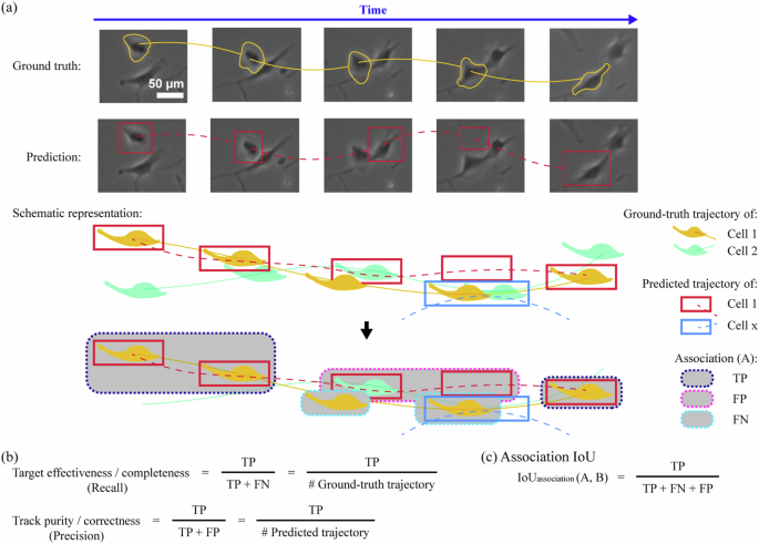
a Schematic representation of cell tracking for ground truth and prediction. b Computational metrics for cell tracking include but are not limited to target effectiveness/completeness, track purity/correctness, and association IoU. Abbreviation: IoU intersection over union.

Full size image

As an alternative means of assessing the performance of such algorithms, various types of biology-associated cell instance segmentation and tracking metrics are employed. For segmentation tasks, common metrics used include whether the number of cells⁷⁶, cell size⁷⁶, and cell centroids^41,81 have been correctly predicted. Such metrics can be directly associated with biologically relevant interpretations. For example, accurate quantification of cell counts, sizes, and centroids as a function of time are informative of cell proliferation, growth, and migration, respectively. For tracking tasks, common metrics used include complete tracks, track fractions, branching correctness, and cell cycle accuracy^44,47,80. Similar to frequently used computer vision-based metrics, these tracking assessment range in values from 0 to 1, representing 0 to 100% performance. Complete tracks compute the fraction of reference annotation cell tracks that can be reconstructed in its entirety and is informative where biological questions pertaining to cell lineage is vital^44,47,80. Track fraction averages the proportion of correctly predicted cell trajectories with respect to the reference annotation and is useful in cell migration analysis^44,47,80. Branching correctness and cell cycle accuracy measure the accuracy of mitosis detection and cell cycle length, respectively, which are indicators of population growth^44,47,80. Thus, various performance metrics associated with frequently sought after biological readings can be used to assess cell instance segmentation and tracking algorithm performance.

In addition to computer vision-based and biological metrics, it is also worth considering usability-driven and carbon footprint-oriented measures. Usability-driven measures are largely concerned with ease-of-deployment (i.e. how rapidly and easy to generate cell instance segmentation and tracking results), including the time to train/execute an algorithm, algorithm complexity in terms of number of tuneable parameters, and generalisability in terms of performance on a similar dataset with the provided parameter settings^44,47. For the former two usability measures, a faster time and smaller number of tunable parameters are indicators of high usability. For the latter, Ulman et al. computes generalisability as the average of SEG and TRA scores obtained on a similar set of image sequence(s) with assessment values ranging from 0 to 1, representing 0 to 100% generalisability in technical performance^44,47. Carbon footprint-oriented measures seek to track energy consumption in the course of developing machine learning models for reducing the environmental impact of such work^82,83. Typically, energy consumption in terms of kWh for different approaches are reported. Such analyses can be monitored using tools such as CarbonTracker⁸² to determine total energy consumption while other tools may breakdown analyses in terms of energy usage by various computer components such as the CPU, GPU, and memory⁸³. Altogether, usability-driven and carbon footprint-oriented measures are gaining recognition as alternate means of assessing cell instance segmentation and tracking performance.

As a comprehensive review of all forms of computer vision segmentation algorithms is beyond the scope of this review, emphasis has been made to explain the inner workings of widely used cell instance segmentation algorithms with the end user (biologist) in mind. This information is presented according to a simple schema that includes traditional/classic non-neural network-based and contemporary neural network-based cell instance segmentation. Readers should note that while various cell instance segmentation metrics associated with different approaches are reported, such performance is highly dependent on individual dataset characteristics and complexity. Therefore, the algorithm performance summarised here may not be generalisable across different datasets and should only be used as a reference.

Numerous traditional/classical cell instance segmentation algorithms have been developed, each with their own strengths and limitations. Traditional/classical algorithms include but are not limited to thresholding, kernel-based techniques, distance transform, watershed, clustering-based approaches, active contour methods, energy minimisation methods, random forest, and support vector machines.

Thresholding involves selecting an optimal value for an image feature such as brightness (i.e. pixel value) and discarding values below this threshold. Typically, cells in ZPCM images have bright halos surrounding them and thresholding may be useful in distinguishing their boundaries. As one of the earliest image segmentation methods, thresholding is rapid to perform but may suffer from problems that it is not generalisable to datasets that are highly variable in nature^84,85,86. Numerous variations on this method exist and may include: local thresholding where subsets of an image are subjected to thresholding based on local image characteristics^84,85, Multi-Otsu thresholding where the histogram of an image’s pixel values is examined and thresholds are automatically computed based on a defined number of categories input by the user⁸⁶, etc. Typically, thresholding may be applied onto less challenging images that have undergone pre-processing. For example, Yin et al. built a mathematical model to approximate the process of ZPCM image formation, which generates restored images of bright cells on a uniformly black background^16,73. These restored images are highly amenable to thresholding and outperformed other computer vision algorithms to attain accuracies of 97.1–90.7% in two separate image sequences^16,73. As such, thresholding is a simple and rapid algorithm that can achieve good cell instance segmentation performance on pre-processed images.

Kernel-based techniques involve applying a matrix or array of numbers called a kernel across an image via a mathematical procedure known as convolution. Briefly, convolution involves the sequential or stepwise sliding of a kernel across the (image) data. During this process, an algebraic operation called the dot product is computed by multiplying each point in the kernel by each corresponding point in the data followed by the summation of these multiplications. This net result of convolution is a filtered image in which a variety of desired effects such as a sharper image, image with fewer noise, etc. is produced.

Within the context of segmentation, convolution results in pattern matching whereby desired image features are extracted and shown as bright pixels against a dark background^84,85. Such filtering may be useful to distinguish cell boundaries via edge detection while shape recognition may be useful in segmenting cells that exhibit a regular shape (e.g. nonadherent cells typically have round morphology). Similar to thresholding, kernel-based image processing is rapid to perform but may suffer from problems in that it is not generalisable to datasets that are highly variable in nature^84,85. Typically, the Laplacian of Gaussian (LoG) or ‘sombrero hat’ kernel is employed owing to its ability to segment binary large objects (blobs; bright regions against a dark background or vice versa)³⁹ but other kernels useful in detecting edges (e.g. Canny, Sobel, etc.) or simple shapes such as rings⁸⁷ may also be used. For adherent cells, their highly variable shape typically contributes towards poor cell instance segmentation performance. Indeed, several variations of cell instance segmentation employing LoG kernels on unreconstructed ZPCM images achieved Dice coefficient ranging from 43% to 52% only³⁹. For nonadherent cells, they typically appear as round objects surrounded by bright halos. Based on these image features, Eom et al. designed a bank of ring filters that achieved 96.5% precision and 94.4% recall on unreconstructed ZPCM images, which outperformed Hough transform—and correlation-based methods.

Thus, kernel-based techniques are simple and rapid algorithms that can achieve good cell instance segmentation performance for non-adherent cells that exhibit regular shapes.

Distance transform is based on the principle that the centre for objects-of-interests i.e. cell centroids are farthest away from the background. This involves devising mathematical criteria for computing the distance of all background pixels to the nearest object pixel or vice versa⁸⁸. For instance, consider the simplest scenario of a binary image where cell regions are given a pixel value of 0 and the background has a pixel value of 1. By computing the Euclidean distance for all pixels in an image with their nearest nonzero pixel, local maxima or peaks will be generated that can be used to separate cells whose boundaries overlap⁸⁸. Similar to thresholding and kernel-based approaches, distance transform is rapid to perform (on binary images) but disadvantages include the requirement for some form of foreground and background segmentation to be performed beforehand as well as its susceptibility for generating numerous false positives^39,88. Numerous variations to address these flaws exist and Dice coefficients ranging from 49% to 80% have been reported on unreconstructed ZPCM images³⁹. A notable variation of distance transform is grey-weighted distance transform, which uses cell shape and intensity information to segment neighbouring or clustered cells with an accuracy rate, positive predictive value, and recall of 97.16%, 98.82% and 98.64%, respectively⁸⁹. As such, distance transform is a useful algorithm that can achieve good cell instance segmentation performance when used in combination with other methods.

The watershed algorithm is a region-based method of segmentation that involves using the image brightness or intensity to create a topographical relief map (bright pixels = high regions whereas dark pixels = low regions) that is subsequently filled or flooded to create distinct regions representing individual objects. The term ‘watershed’ is derived from Geology and refers to the divide which separates adjacent basins, which within this context would typically represent the boundaries of cells. The watershed algorithm is robust and can be applied across different imaging modalities such as ZPCM and fluorescence microscope images but it is prone to oversegmentation (generating too many segments)^39,84,85. As a result, variations such as marker-based watershed have been developed to minimise this issue. In Vicar et al., marker-controlled watershed as a standalone algorithm achieved a Dice coefficient of 41% on unreconstructed ZPCM images, which can be improved to 52% when used in combination with thresholding and distance transform³⁹. Thus, watershed achieves reasonable cell instance segmentation performance when used in combination with other methods.

Clustering algorithms operate on the principle that regions of an image with similar image features belong to the same object. Such image features may include brightness, texture, colour, etc., and numerous variations such as k-means clustering and mean-shift exist^84,85. k-means clustering is a popular choice for segmentation due to its simplicity and operates by first randomly dividing an image into k number of clusters and assigning individual datapoints (feature points) to the nearest mean^84,85. Upon completing this assignment, the mean for each cluster is recomputed and feature points are reassigned^84,85. This latter process repeats until the means no longer move, indicating convergence upon a solution^84,85. However, drawbacks of k-means clustering include requiring the number of clusters to be specified and sensitivity to initialisation conditions^84,85. Such drawbacks can be addressed by using the mean-shift algorithm, which automatically identifies the number of clusters within the data for simultaneous cell instance segmentation and tracking but clever strategies to overcome the model’s slow inference speed must be devised⁹⁰. Owing to the complexities of cell instance segmentation, K-means clustering is typically used in combination with other methods rather than as a standalone approach⁹¹. Such attempts have achieved F1 scores ranging from 90.92% to 96.59% for three different cell types in unreconstructed ZPCM images⁹¹. As such, clustering algorithms can partition image features to achieve good cell instance segmentation performance when used in combination with other methods.

The goal of active contour methods is to segment the boundaries of objects. The algorithm operates by using an enclosed curve as an initial boundary, which then iteratively shrinks or expands according to local differences present in an image^84,85. Two major variations of active contours are the ‘snakes’ and ‘level set’ implementations, which utilise different mathematical approaches to govern the shrinking or expanding movement of the contour^84,85. Since cells have enclosed boundaries, this algorithm is highly suited for their segmentation. The advantage of this method is the generation of sub-regions with continuous boundaries in contrast to kernel-based edge detection methods which may produce discontinuous or interrupted boundaries^84,85. However, ideal parameters must be identified to ensure accurate performance as it has been noted that the contours tended to shrink too much when used to segment cells³⁹. When used to perform semantic cell segmentation, various implementations of level-sets attained Dice coefficients ranging from 64% to 77% on unreconstructed ZPCM images³⁹. Thus, active contour methods can achieve good semantic cell segmentation performance.

Energy minimisation methods formulate images in terms of an energy function and implement an algorithm that minimises this energy, resulting in the efficient partitioning or segmentation of an image. Numerous variations of energy minimisation methods exist with graph-based segmentation or ‘graph cuts’ being widely used^84,85,92.

Specifically, images may first be formulated as graphs by substituting a vertex for each pixel, connecting an edge between each pair of pixels, and assigning a weight for each edge based on the affinity or similarity between two vertices^84,85. Image segmentation occurs by implementing as minimal number of cuts within the graph as possible such that each partitioned subgraph only contains vertices that have high affinity for each other^84,85. This typically results in good performance when performing binary cell (foreground) and background segmentation but segmentation with multiple (more than 2) labels may prove problematic. Also, by implementing a minimal number of ‘graph cuts’, the algorithm may not work well for segmenting thin structures involved in cytoplasmic processes^84,85. Indeed, implementation of ‘graph cut’ algorithms is typically reserved for semantic segmentation, achieving a Dice coefficient of 40–86% on unreconstructed ZPCM images. However, Bensch et al. utilised a min-cut approach to generate cell instance segmentation masks. This method leveraged on the principle that a cell’s true boundaries in positive ZPCM consistently manifests as a transition from dark to bright in an outward direction⁹². With this approach, an average segmentation score of 81.05% was achieved on two ZPCM image sequences⁹².

As such, energy minimisation techniques such as ‘graph cut’ are typically employed for semantic segmentation but can also achieve good cell instance segmentation performance.

The random forest algorithm is a supervised (learning) classifier that is comprised of a collection of decision trees, operating on the tenet that the collective decision of a diverse group of independent trees is superior to the opinion of a single tree. Implementation of a random forest requires providing labelled data on relevant image features, which are used to build a random collection of decision trees^84,85. This requirement to provide relevant image features is termed feature engineering and is crucial to performance. Poorly engineered features may not contribute towards increased performance and may instead decrease performance^84,85. When constructed, each individual decision tree can produce a prediction (the equivalent of a vote) with respect to the classification task and the majority vote determines the final collective classification outcome^84,85. This classification task can be a simple binary decision such as determining whether an image pixel is foreground (cell) or background (non-cell) to slightly more complex non-binary classifications such as whether pixels belong to a cell, mitotic cell, halo, or background noise^84,85,91. Following this, the prediction may be further processed in combination with clustering and other classification algorithms to achieve versatile segmentation (87.66–95.98% precision and 94.43–97.20% recall) of mouse NIH3T3 fibroblasts and human U2OS bone epithelial cells in unreconstructed ZPCM images⁹¹. Thus, random forest algorithms can achieve good performance when used in combination with other methods.

Support vector machines (SVMs) are a set of supervised learning methods that can be used in classification, regression, and outlier detection. SVMs operate by transforming the data onto a higher dimension and finding an optimal decision boundary known as a hyperplane that reliably separates the labelled data according to their groups^84,85. Similar to the random forest algorithm, explicit feature engineering is required and if ideal image features are selected, good performance can be attained^84,85. SVMs also have the benefit of being effective in high dimensional space, but it may require longer computational times to train for large datasets^84,85. For example, Pan et al. used a SVM to learn image features associated with variations in cell appearances and shapes while maintaining its ability to discriminate against non-cell background⁹³. Specifically, following a series of pre-processing steps, candidate cell centroids are identified and the regions surrounding these cell centroids are subjected to image feature extraction⁹³. These image features include attributes associated with cells in ZPCM images such as the bright halo artefacts and the spatial presence of edges⁹³. A SVM is used to distinguish between cell and background pixels and a further series of steps is taken to determine whether pixels belong to the same cell before grouping them accordingly⁹³. This resulted in a F1 score of 90.0% for mouse C2C12 myoblasts and bovine aortic endothelial cells⁹³. As such, SVM is a useful algorithm that can achieve good and versatile cell instance segmentation performance when used in combination with other methods.

Numerous traditional/classical algorithms including thresholding, kernel-based techniques, distance transform, watershed, clustering-based approaches, active contour methods, energy minimisation methods, random forest, and support vector machines have been developed. Although these algorithms utilise different methodologies, they share in common that image features are explicitly extracted or engineered via expert domain knowledge. Some of these algorithms may either operate on a standalone basis or need to be used in combination with others if they only excel at specific tasks such as semantic segmentation. Overall, these algorithms may attain metric scores as high as 97% but care must be taken when interpreting the versatility of these results as algorithm performance may be dependent on image complexity.

Numerous artificial neural network-based or deep learning computer vision cell instance segmentation algorithms have been developed, each with their own strengths and limitations. An artificial neural network is inspired by synapses of the brain and is comprised of groups of interconnected nodes, analogous to neurons, which are organised into three types of layers^94,95,96. These three layers include: (i) an input layer, where the data is initially loaded into the model, (ii) hidden layers, which perform various computations such as extracting features and representations from data, and (iii) the output layer, which takes the preceding output of hidden layers to generate a final prediction^94,95,96. The nodes and connections of an artificial neural network are referred to as artificial neurons and edges, respectively^94,95,96. Each artificial neuron receives an input, performs a simple computation, and transmits an output via its edge^94,95,96. Various weights are typically associated with each artificial neuron and edge^94,95,96. During development of a deep learning model, these weights are adjusted according to the labelled (training) data provided such that the model can learn the statistical distribution of the data and make accurate predictions when called upon^94,95,96. As previously mentioned, deep learning computer vision algorithms differ from traditional/classic non-neural network in that image features and representations are not explicitly extracted or engineered by an expert with domain knowledge. Rather, these image features and representations are learned and computed within the hidden layers of the artificial neural network, which do not require expert input as long as sufficiently appropriate and high-quality labelled data is provided for model training. Thus, deep learning algorithms come in numerous subvarieties and those relevant to cell segmentation include but are not limited to convolutional neural networks (CNNs), recurrent neural networks (RNNs), and transformer neural networks.

CNNs are deep learning architectures that are well adapted for spatial data such as images, in part, due to a specialised type of hidden layer known as the convolutional layer^94,95,96. Similar to kernel-based techniques, the convolutional layer of CNNs utilises kernels to identify the presence of relevant image features or patterns^94,95,96. However, these kernels do not need to be explicitly specified and higher ordered representations of image features can be identified by a CNN’s successive (deeper) hidden layers^94,95,96. For example, a relatively shallow hidden layer may identify a low tier feature such as a line or edge that signifies part of an object boundary whereas a relatively deeper hidden layer may utilise the outputs of several shallow hidden layers to identify higher tier features such as complex shapes that represent a part of the cell such as its nuclei or complete cell boundary^94,95,96. Numerous variations of CNNs exist with several state-of-the-art architectures, UNet⁹⁷, CellPose^98,99, StarDist¹⁰⁰, and MaskRCNN^80,101, being widely used in biomedical imaging and computer vision applications, respectively. UNet is a CNN model that is primarily used for semantic cell segmentation. However, variations of this model can achieve instance cell segmentation by using UNet models to predict cell cytoplasm and background (2-class UNet) or cell cytoplasm, background, and cell borders (3-class UNet). Such efforts have resulted in mean IoU scores of 63.3–92.4% on unreconstructed ZPCM images⁹⁷. CellPose uses a variation of the UNet architecture to predict a combination of vertical and horizontal image gradients. These image gradients are important feature of images and can be used to delineate the centre of an object to its edges/borders. This algorithm has been effectively used for generalised cell instance segmentation for non-fluorescent and fluorescent images, achieving an average precision of 0.77 (IoU threshold = 0.5) on generalised data^98,99. On a similar variation of this theme, StarDist use a simple UNet model to predict star-convex polygons, which are well-suited to approximate the shapes of nuclei and cells, and has demonstrated an average precision of 86.41–99.84% for nuclei and cell images¹⁰⁰. MaskRCNN is a CNN model that is primarily used for instance cell segmentation. This model has a region proposal network that first predicts a boundary box that encloses the object of interest along with the category/class label of the object. Subsequently, a binary mask is then predicted for each object enclosed within the initially predicted bounding box. MaskRCNN has been used on unreconstructed ZPCM images with mean IoU scores of 72.1%^80,101. Thus, CNNs such as UNet, CellPose, StarDist, and MaskRCNN are well suited to achieve good semantic or instance cell segmentation performance.

Recurrent neural networks (RNNs) are architectures that are well adapted for sequential or temporal data, in part, due to a specialised type of hidden layer known as the recurrent layer^94,95,96. Unlike most artificial neural networks which operate in a linear-wise manner, the recurrent layer of RNNs can receive two types of input—its immediate current input (similar to typical artificial neural networks) and preceding inputs from recent past. This allows the recurrent layer to retain a memory of current and prior inputs, allowing them to influence the computation of its output^94,95,96. This attribute makes RNNs adept at processing sequential or time series data and several variations including long short-term memory networks (LSTM) and combined CNN-RNN models have also been developed. For example, Arbelle and Raviv incorporated convolutional LSTM blocks into a UNet model in order to take advantage of their combined ability to extract meaningful spatiotemporal information including the ability to consider past cell appearances via its LSTM memory units¹⁰². This resulted in a Seg score of 27.0–85.9% and Det score of 74–98.2% although a recent 2021 version of this algorithm showed a Seg score of 64.1–92.2% and a Det score of 96.1–99.0%^78,102. Thus, RNNs can achieve good instance cell segmentation performance.

Transformer neural networks are deep learning architectures that are well suited for both spatial or sequential data, in part, due to a specialised type of hidden layer known as the attention layer^{94,95,96,103,104}. Briefly, the attention layer models biological cognitive attention by assigning different weights to a sequence of inputs, with higher weights denoting higher emphasis or attention to that specific portion of the overall input. In the case of vision-based transformers, an image may be reformatted into a sequence of sub-images or sub-crops termed patches. This attribute makes transformer neural networks highly versatile for processing spatial or sequential data although current state-of-the-art models typically require much more data than CNNs for model training to attain good performance. Despite this, transformer neural networks have been used to achieve instance segmentation of yeast cells in brightfield microscopy with a mean IoU score of 84–85%¹⁰⁵ as well as average precision of 87% and recall of 91% for immortalised human lung epithelial cells in a wound repair dataset¹⁰³. As such, transformer neural networks hold potential for cell instance segmentation algorithms in ZPCM images.

Numerous contemporary neural network-based algorithms including CNNs, RNNs, and transformer neural networks have been developed. Although these algorithms utilise different methodologies, they share in common that they are domain-agnostic, with image features and representations implicitly extracted and learned via labelled data. Overall, these algorithms may attain metric scores as high as 99% but similar to traditional/classical algorithms, care must be taken when interpreting these results since algorithm performance varies with different image complexities.

Similar to cell segmentation algorithms, widely used cell tracking algorithms are presented according to the dichotomy of traditional/classic non-neural network-based and contemporary neural network-based cell segmentation. Notably, several tracking algorithms utilise similar methodologies as cell segmentation algorithms, and therefore discussion of their inner workings are kept to a minimum. Generally, cell tracking algorithms operate via two guiding principles: (i) tracking-by-detection, whereby cell segmentation is performed for every frame in an image or video sequence followed by association between frames to generate cell tracks or trajectories or (ii) contour-based methods, in which cells are initially segmented in the very first frame of an image or video sequence and the boundaries of each segmented cell used to initiate segmentation in the subsequent frame while simultaneously performing tracking^{44,80,106,107,108,109,110}. As tracking algorithms can apply beyond the scope of cell tracking, particularly for the tracking-by-detection paradigm where segmentation and tracking tasks are clearly separated with little-to-no overlap, the discussion below is limited to specific examples associated with cell tracking. Similar to cell instance segmentation algorithms, the cell tracking performance reported herein should only be used as a general guide given that similar results cannot be guaranteed across different datasets.

Numerous traditional/classical cell tracking algorithms have been developed, each with their own strengths and limitations. Traditional/classical algorithms include but are not limited to distance-based nearest neighbour linking, motion-based tracking, clustering-based mean shift tracking, active contour-based level set methods, energy minimisation-based graph association, and global spatiotemporal association approaches^{44,74,75,78,90,103,106,111,112,113,114,115}.

Briefly, the specific methodology and performance for the above-mentioned methods are described as follows. As implied by its name, distance-based nearest neighbour linking computes the shortest distances for a group of cells and their new candidate positions in the next successive image or video frame^44,78. Numerous variations of the method exist with algorithms in the cell tracking challenge dataset achieving TRA scores of 4.0–98.5%^44,78.

Similarly, motion-based tracking may make use of various motion features to create cell trajectories¹⁰³. For example, Gwatimba et al. developed a custom algorithm that extracted four motion-based features based on IoU, Euclidean distance, motion vectors, and temporal distance, achieving a TRA score of 0.5 for DIC microscope images in the cell tracking with mitosis detection challenge dataset¹⁰³.

In clustering-based mean-shift tracking, the mean-shift algorithm is used to cluster extracted image features and representations that distinguish cells across an image or video sequence^90,113. For example, Letort et al. utilised their algorithm to shift and converge concentrically arranged triangle-shaped kernels towards regions containing a specific mix of dark and bright regions, since cells within ZPCM images appear as dark objects surrounded by bright halos¹¹³. This approach resulted in minor cell positional discrepancies (about half a cell diameter or 26 µm) between manual and automated methods as well as a low proportion (4.2%) of cells that were deemed to be ‘lost’ when tracked by their algorithm¹¹³.

In active contour-based level set methods, the boundaries of segmented cells are ‘evolved’ such that they not only match the cell appearance in the current frame but can conceivably match candidate cell regions across other frames based on image features and motion predictions¹¹⁴. This work generated a high overall percentage (88.4%) of valid cell trajectories¹¹⁴.

In energy minimisation-based graph association, similar to its cell segmented counterparts, cell tracking is accomplished by formulating the task as a graph-based optimisation problem and attaining the solution at a minimum cost. Such algorithms have achieved TRA scores of 95.9–97.7% in the cell tracking challenge dataset^44,78.

In global spatiotemporal association approaches, temporal information from the overall sequence is considered in order to generate reliable cell trajectories and reduce errors^106,111. For example, an approach that only assigns cell trajectories over a relatively long duration will fare better against a short duration as false positives generated as a result of segmentation errors will typically disappear after several frames^106,111. By hypothesising all possible cell trajectories as branching tree structures (so as to account for cell division), the ideal solution was found via linear programming and resulted in a target purity of 81% and target effectiveness of 87%^106,111

Numerous artificial neural network-based or deep learning computer vision cell tracking algorithms have been developed, each with their own strengths and limitations. Deep learning algorithms come in numerous subvarieties and those relevant to cell tracking include but are not limited to CNN-, RNN-, Siamese-, and Graph neural network (GNN)-based tracking. Briefly, the specific methodology and performance for the above-mentioned methods are described as follows.

In CNN-based tracking, the strength of using convolutional operations can be leveraged to detect visual and spatial features in an image sequence¹¹⁶. For example, Chen et al. integrated an additional cell tracking branch into the architecture of the MaskRCNN model such that it can detect spatial and visual features associated with cell positioning and cell appearances, respectively¹¹⁶. Within the context of cell tracking, spatial features are of particular importance to tracking accuracy since there are numerous cells with similar appearances, making visual information alone insufficient for identifying the same cell across different timepoints. However, when labelled successive frames (i.e. the previous and current timepoints) are used as training input, the model learns spatial features and representations associated with cell positions¹¹⁶. These learned features and representations enable the model to generate a similarity score for candidate pairs of cells across successive timepoints that determines if they are the same cell or not¹¹⁶. This allowed the algorithm to achieve a TRA score of 97.05% in the DeepCell dataset¹¹⁶. Indeed, the importance of these spatial features was demonstrated in an ablation study whereby removing parts of the model associated with spatial feature detection decreased the TRA score by 2.86%¹¹⁶.

In RNN-based tracking, the strength of using recurrent operations can be leveraged to parse temporal image sequences. For example, Kimmel et al. developed a CNN-based model equipped with recurrent LSTM units to implicitly represent the temporal dimension¹¹⁷. By training the model on 20 time steps of motion and predicting 10 time steps into the future, the RNN model produced an average mean squared error of 192, which was lower than the average mean squared error of 220 achieved by a baseline kinematic model¹¹⁷.

In Siamese tracking, two identical neural networks, typically CNN-based, are utilised to extract features and data representations from two inputs for comparison¹¹⁸. Since both neural networks utilise identical parameters, they can be trained to assess whether both inputs are similar¹¹⁸. Within the context of cell tracking, a Siamese tracker can be used to match the location of the same cell across successive frames (i.e. along the temporal axis)¹¹⁹. Using a combination of a UNet model and watershed algorithm for initial segmentation, Panteli et al. employed Siamese tracking to determine if cells were ‘colliding’ (i.e. coming into close proximity), participating in cell division, or undergoing cell death¹¹⁹. Based on the Siamese tracking output, cells were re-segmented as necessary using the watershed algorithm¹¹⁹. This approach reduces false positives and negatives that may originate from over- and under-segmentation, allowing a TRA score of 0.966 to be achieved in phase contrast time-lapse sequences¹¹⁹.

In GNN-based tracking, the entire microscopy image sequence is formulated as a direct acyclic graph such that cell instance segmentation results and their associated cell trajectories are represented by graph nodes and their associated vertices edges, respectively¹²⁰. This formulated graph represents all possible trajectory solutions and the objective is to identify a subgraph that optimally reduces tracking errors while accurately representing cell trajectories and behaviours such as cell division and cell death¹²⁰. GNNs can be implemented in a variety of ways, and may contain elements derived from CNNs, RNNs, or transformer neural networks^121,122. In Ben-Haim et al., a GNN employing an edge-attention mechanism attained TRA scores of 0.985 on a phase contrast microscopy image sequence¹²¹.

Several key considerations that affect algorithm development and performance relate to handling of cell overlaps, implementation of specialised tracking system modules such as mitosis detection, use of objective benchmarking, application of semi-automated frameworks, and elucidation of operating mechanisms behind learning-based algorithms.

Cell overlaps occur when two or more cells come closely into proximity in a manner that obscures intercellular boundaries, negatively impacting the precision of individual cell instance segmentation and their resulting trajectories. Such scenarios may occur when neighbouring cells are grown at high densities, in migration studies when cells may crawl over one another, as well as in cell types such as neurons whose long and thin cytoplasmic processes may partially extend over nearby cells^{123,124,125,126,127,128,129,130}. Cell instance segmentation errors from these scenarios often result in cell misidentification, which further compound mistakes in cell tracking and subsequent computation of cell lineages¹²⁴. Of note, this concept should not be confused with overlap-based cell tracking, in which a high degree of cell mask overlap between consecutive frames in a time-lapse sequence or video is useful for inferring correct cell tracking trajectories^44,47,131. Handling of cell overlaps may be in-built into an algorithm’s output and implementation. To handle cell overlaps via algorithmic output, certain cell instance segmentation software may only allow an image pixel to be associated with a single cell mask^98,99 whereas others permit association with multiple cell masks^80,101. In the latter case, this more accurately depicts a real-world 3D scenario in which a cell or part of a cell has overlapped with its neighbour, thus preserving information that may be useful for subsequent cell tracking. To handle cell overlaps via algorithmic implementation, several traditional/classic non-neural network and contemporary neural network-based approaches have been utilised^{123,124,125,126,127,128,129,130}. These include using Gaussian mixture models to model cell clusters¹²⁵, random forests that select image features for classifying between overlapping and individual objects¹²⁸, contour-based methods that model cell clustering scenarios to distinguish individual cell boundaries^124,126, and CNNs that use a distance map penalty function to focus attention on dense cell clusters¹²³. Therefore, cell overlaps represent a major impediment for precise cell instance segmentation and tracking performance, requiring specific algorithmic output and implementation to address them.

In addition to identifying the same cell across different timepoints, tracking systems may also incorporate specialised tracking modules for handling special circumstances or exceptions that result in the appearance, disappearance, and morphological changes of cells. For example, events associated with the sudden appearance of new cells include cells migrating into the microscope’s current field of view or a mother cell dividing into two daughter cells whereas the sudden disappearance of cells include cells migrating out of the current field of view or cell death. In addition, cells may undergo dramatic morphological changes during differentiation as well as disappearance. As such, devising algorithms that detect cell behaviours such as apoptosis or cell death¹³², mitosis or cell division^{111,132,133,134,135,136}, and cell differentiation¹³⁷ will be useful for handling these special exceptions. Traditional/classical non-neural network algorithms for these tracking modules may utilise SVM^132,133 and tree¹¹¹ methods whereas contemporary neural network-based algorithms may include CNNs¹³⁴, CNN-RNN hybrids¹³⁵, and deep reinforcement learning¹³⁶. Together, employing such specialised modules within a tracking system can improve overall cell instance segmentation and tracking performance.

As noted previously, image complexity and computer vision can greatly impact algorithm performance. Therefore, it is crucial that algorithms are objectively compared on the same datasets in order to determine their robustness and versatility. Based on objective benchmarking comparisons conducted by Vicar et al. ³⁹ and Ulman et al. ⁴⁴, several key points related to algorithm development and performance have been identified, namely that (i) image reconstruction improves cell segmentation^39,44, (ii) cell detection methods employing contemporary supervised learning are typically superior to other approaches⁴⁴, (iii) tracking-by-detection typically outperform contour-based methods although contour-based methods tend to generate more stable (i.e. longer) cell trajectories⁴⁴, and (iv) methods that use prior and contextual biological information typically perform better than those that do not⁴⁴. Thus, objective benchmarking has identified that algorithms employing image reconstruction, contemporary supervised learning, tracking-by-detection paradigm, and incorporating prior or contextual biological information can result in enhanced performance.

Despite numerous significant advances, the performance of fully automated cell instance segmentation and tracking algorithms are suboptimal relative to manual tracking. Indeed, this has necessitated software for error corrections¹³⁸ and disclaimers that none of the top performing algorithms in cell instance segmentation and tracking competitions may be satisfactory ‘when judged from a biologist’s viewpoint’⁴⁴. Within this context, semiautomated frameworks may be ideal compromises between tedious manual but reliable tracking with rapid but error-prone automated computer-based tracking¹³⁹. For this reason, there have been semi-automated pipelines where humans and algorithms work in tandem to either generate accurate labelled data such as cell segmentation annotations⁴⁵ or aid the user in curating cell tracking data¹³⁸. Thus, semi-automated pipelines may prove a valuable approach in development of next-generation cell instance segmentation and tracking software.

In addition, despite their outstanding performance, a well-established view of contemporary neural network-based methods is that they operate as black boxes as it is not immediately clear what image features are being computed within the hidden layers. To address this issue, a variety of computational tools have been developed to elucidate the inner workings of artificial neural networks. Such tools include pixel attribution approaches or saliency maps¹⁴⁰, which can be used to visualise important image features that may explain how neural networks arrived at a decision. After the methodology of an artificial neural network is understood, it may be possible to develop improved versions of algorithms for both cell instance segmentation and tracking. Such efforts may also involve merging classical segmentation algorithms, which are based on solid mathematical foundations together with contemporary neural network-based approaches.

Altogether, the presence of specialised tracking modules, choice of algorithm and tracking paradigm along with software that incorporate human input as well as attaining clearer understanding of how algorithms operate are vital considerations for algorithm development and performance.

In summary, cell instance segmentation and tracking algorithms can be categorised according to whether image features and representations are explicitly defined or extracted. Within this schema, a diverse variety of traditional/classic non-neural network and contemporary neural network-based cell instance segmentation and tracking algorithms have been developed with varying performance. Vital considerations that influence performance include whether image pre-processing such as image reconstruction are performed along with the type of algorithm(s) and paradigm used for cell instance segmentation and tracking. This may include whether specialised cell instance segmentation and tracking modules as well as semi-automated frameworks are used. With careful consideration of these issues, both algorithm developers and end users can foster the development of novel algorithms with high cell instance segmentation and tracking performance as well as the generation of reliable biological interpretations.

Given that label-free microscopy can easily generate cell instance segmentation and tracking data with relatively simple, low-cost equipment that offers powerful, multiple biological readouts at the single cell and population level, a crucial factor that limits their widespread use is the performance of cell instance segmentation and tracking algorithms for universal recognition of cells. Below we outline potential areas that may further accelerate algorithm development and performance in terms of (limited) availability of annotated datasets as well as recent software advances (cell instance segmentation and tracking algorithms). Furthermore, emerging trends in utilising existing cell instance segmentation and tracking algorithms for novel purposes and within more physiologically relevant 3D systems are discussed.

Data are indispensable for evaluating algorithmic performance and training machine learning-based models. Typically, larger datasets result in greater performance of machine learning-based models. While traditional machine learning algorithms typically exhibit a performance curve that increases with more data according to a power law, this eventually reaches plateau. Conversely, it has been reported that neural network-based models exhibit increased performance in a logarithmic manner with increased data size¹⁴¹. In that respect, well-annotated, large datasets are vital to algorithm performance. As previously mentioned (Data Generation and Cell Annotation Curation), obtaining high quality curated image data can be laborious, expensive, and highly time consuming^41,44,142. In this regard, large microscope datasets have been published in recent years (Table 8), which include over 1.6 million human annotated cells imaged with a 10× magnification objective¹⁴² as well as over 1 million human annotated and about 10 million computer tracked cells imaged with a 5× magnification objective⁴¹. Such datasets will prove highly useful for algorithm development. Importantly, it is worth noting that datasets are not completely free of errors as even experts may also mislabel data, which may impact both model development and performance assessment (https://labelerrors.com)¹⁴³.

Accordingly, ingenious ways to maximise data usage is necessary. Several such strategies may include: (i) developing learning-based algorithms that maximise efficient usage of datasets¹⁴⁴ such as training on multimodal data to improve task performance¹⁴⁵, (ii) data augmentation, (iii) transfer learning¹⁴⁶ using publicly available image datasets of cells that are derived from various microscope modalities (Table 8)^147,148, and (iv) generating synthetic images¹⁴⁹ from self-generated or publicly available datasets (Table 8).

Together, these strategies may overcome microscope image data sparsity or leverage on existing public datasets to attain excellent cell instance segmentation and tracking performance.

While it is inevitable that cell instance segmentation and tracking algorithms will advance with time, their progress can be accelerated by the advent of novel model architectures and algorithms, international competitions, and use of biological metrics. For example, transformer neural networks are a relatively new type of model architecture and reportedly required fewer parameters and ran 30% faster while matching the segmentation performance of state-of-the-art MaskRCNN recognition of cells under relatively simplistic scenarios¹⁰⁵. Also, novel algorithms that operate on incomplete information or sparse labels i.e. data with only cell centroid labels as opposed to cell mask labels have been reported for both cell segmentation¹⁵⁰ and cell tracking¹⁵¹. In addition, there are efforts aimed at developing algorithms that are capable of exhibiting few shot learning or using a limited number of examples to generate a well-generalised model¹⁵². Indeed, such algorithms can reduce the burden of data collection and curation. In addition, open competitions have been held to encourage further innovations in the field. For instance, the Cell Tracking Challenge (http://celltrackingchallenge.net/)¹⁰⁵, often organised in conjunction with the international symposium on biomedical imaging (ISBI), aims to spur innovation in instance segmentation and tracking of cells or subcellular structures across multiple imaging modalities including ZPCM, DIC microscopy, and fluorescence microscopy. Meanwhile, other competitions such as the Data Science Bowl (37,333 manually annotated cell nuclei; https://www.kaggle.com/c/data-science-bowl-2018)¹⁵³ aims to prompt automated segmentation of cell nuclei for enhancing biomedical research. Subsequent head-to-head comparisons of such algorithms^44,153, despite being geared towards more general algorithms that can recognise across different image modalities (e.g. fluorescence, brightfield, etc.), will undoubtedly spur additional algorithm development and innovation.

As end users, biologists and biomedical researchers have specific scientific questions that they wish to answer. At present, it has been acknowledged that current state-of-the-art for label-free cell segmentation and tracking produces less than desirable results for extracting biologically meaningful interpretations⁴⁴. Indeed, Maier-Hein et al. ⁷⁶ and Reinke et al. ¹⁵⁴ have highlighted the great chasm between algorithm development and its translation into practice owing to a poor choice of computer vision metrics. In this regard, they have developed a framework entitled ‘Metrics Reloaded’ that can be accessed online (https://metrics-reloaded.dkfz.de/) to guide users on selecting appropriate metrics while considering the biological or biomedical need, mathematical properties of metrics, or attributes of the specific data set⁷⁶. In addition to these efforts, it may be crucial for computer vision scientists to begin adopting biologically derived metrics to validate their algorithms. Notably, biological metrics derived from cell tracking are highly sensitive to errors that occur early on, which compound mistakes to generate incorrect study interpretations. Therefore, modification of existing algorithm performance metrics to emphasise accuracy from time zero (e.g. proportion of correctly tracked cells from time zero) would encourage computer vision scientists to pay attention towards developing algorithms that do not make early mistakes. In addition, such time-associated tracking metrics would allow biologists and biomedical researchers to quantitatively assign a level of confidence to experimentally derived interpretations.

Thus, the advent of novel model architectures and algorithms, open international competitions, and use of biological metrics to validate algorithm performance is expected to accelerate versatility and performance of existing cell instance segmentation and tracking algorithms.

Beyond existing efforts to accelerate algorithm development and performance, there are also new emerging trends resulting from novel applications of cell instance segmentation and tracking algorithms for 3D live culture studies as well as multiplexing of cell imaging data with omics-based analyses.

To better mimic physiological relevance, there have been efforts to apply cell instance segmentation and tracking algorithms on label-free 3D live cell cultures. Such endeavours require an imaging modality with good optical sectioning capabilities and accurate curation of cell reference annotations. Typically, imaging modalities such as brightfield microscopy¹⁵⁵, DIC microscopy¹⁵⁶, or ZPCM¹⁵⁷ are used given their widespread ubiquity although 3D imaging techniques based on holographic tomography principles¹⁵⁸ and third harmonic generation¹⁵⁹ have also been reported. Acquisition of 3D cell data face similar challenges as 2D in vitro models but entail an added level of complexity owing to their 3D nature. This is because thicker specimens tend to result in more pronounced artefacts such as out-of-focus background light from different image planes¹⁵⁹, image blurring due to undesired optical diffraction⁴⁰, and image intensity variations from inhomogeneous illumination or light absorbing obstructions such as extracellular matrix^40,155. These factors contribute towards the highly challenging nature of manually generating 3D cell reference annotations. In addition, curation of 3D data requires investment of tremendous amounts of resources. For example, a cell that spans 30 slices would take 30 times longer to manually segment in 3D than in 2D⁹⁹. As a workaround, studies have resorted to objective labels such as fluorescent dyes to improve both curation and development of cell instance segmentation and tracking algorithms. Ultimately, while such workarounds may utilise fluorescent labels that cause undesired phototoxicity and photobleaching¹⁵⁵ during development of a cell instance segmentation and tracking system, the trained model can remain label-free after supervised learning¹⁶⁰. Therefore, 3D live cell imaging data typically utilise similar imaging modalities as their 2D counterparts but entail a higher level of complexity and challenges in terms of both data acquisition and curation.

Given shared use of the same imaging modalities, it is not surprising that similar cell instance segmentation and tracking algorithms are used in both 2D and 3D live cell cultures. These include 3D versions of traditional/classic non-neural network-based and contemporary neural network-based algorithms based on thresholding, template matching, distance transform (e.g. geodesic), watershed, active contours (e.g. snakes and level set), energy minimisation (e.g. graph-based), random forest (e.g. Tree Bagger), SVMs, CNNs (e.g. 3D U-Net, MaskRCNN, CellPose), and various pipelines utilising various algorithmic combinations^{40,155,161,162,163}. For the sake of brevity, readers are referred to excellent reviews and benchmarks by Hollandi et al. ¹⁶³, Kar et al. ⁴⁰, and Carvalho et al. ¹⁶². Alternatively, 3D live cell data that are image stacks of 2D slices can undergo 2D cell instance segmentation and tracking followed by stitching to produce a reconstructed 3D volume. Both CellPose^98,99 and CellStitch¹⁶⁴ are recent examples that exhibited good cell instance segmentation performance in terms of biological (i.e. cell numbers) and computer vision (precision, recall, average precision, and mean average precision) metrics, respectively. An advantage of this approach is that 2D stitching can leverage upon the availability of existing 2D cell instance segmentation datasets, which are more plentiful and diverse than current 3D training datasets¹⁶⁴ and also require less computational resources such as GPU memory to run¹⁶⁵. Thus, 3D live cell cultures utilise similar cell instance segmentation and tracking algorithms as their 2D counterparts.

Using such cell instance segmentation and tracking algorithms, studies have demonstrated the promise of performing label-free image analysis on patient-derived spheroids and organoids for drug discovery^166,167. For example, Deben et al. developed a convolutional neural network that used brightfield images as input and trained on fluorescent images as output. Once the model was trained, the system was label-free, requiring only brightfield images to make predictions. This system was used to screen for chemotherapeutics on patient-derived organoids and showed comparable performance as CellTiter-Glo 3D, a gold standard analysis method¹⁶⁶. In addition, the predicted responses were used to improve patient stratification, allowing for better drug response estimates, and is currently being trialled in a larger patient cohort¹⁶⁶.

To further extend the scope of biological inferences derived from cell instance segmentation and tracking predictions, Cutiongco et al. computed various morphological attributes for predicting gene expression¹⁶⁸. These morphological parameters included geometric measurements (e.g. area, perimeter, radius, etc.), textural measurements such as Gabor features, granularity, intensity measurements, and radial distribution measurements (e.g. Zernike shape features)¹⁶⁸. When several stem/progenitor cell lines were cultured on top of nanotopographical patterns, accurate gene expression level predictions were achieved for 14 different genes, enabling the effect of cell response to nanotopographical substrates to be studied¹⁶⁸.

In summary, label-free cell instance segmentation and tracking in label-free live cell microscopy is expected to benefit from the availability of more curated datasets, strategies that maximise data usage, development of novel computer vision models and algorithms, benchmarking of algorithms in international competitions, and formulation of biologically relevant performance metrics that enable biologists and biomedical researchers to make sound interpretations of their studies. Recent emerging trends seek to expand the frontiers of this field by applying label-free cell instance segmentation and tracking algorithms in more physiological 3D systems such as patient-derived organoids for drug screening and utilising computed biological metrics for predicting gene expression.

As an inexpensive and ubiquitous bioimaging modality, label-free live cell microscopy is an ideal technique for label-free instance segmentation and tracking of cells, with enormous potential for numerous basic and translational applications. The workflow for data generation is straightforward with low requirements in terms of microscope and computer hardware, allowing the rapid generation of large volumes of cell images. From these cell images, numerous biological metrics for a cell population of interest can be attained with single cell resolution to robustly answer numerous scientific questions. A grand challenge remains in developing computer vision-based models and algorithms that can accurately and rapidly segment and track cells, which currently comprise of various traditional/classic non-neural and/or contemporary neural networks. Such challenges may be addressed from a software perspective by increased availability of new datasets or development of novel computer vision models/algorithms as well as from a hardware perspective by advances in alternative label-free technologies. Altogether, label-free cell instance segmentation and tracking using microscope-based methods holds significant potential for advancing our understanding of biology and human health.