Landslide-channel feedbacks amplify channel widening during floods
Introduction
Flood stream power is amplified in mountainous catchments by channel confinement and steep slopes, generating widespread channel erosion and causing substantial challenges for flood risk management in these regions. Approaches to predicting flood channel response include identification of stream power thresholds1,2, duration of flow above a critical value3, and downstream gradients in stream power4. However, other studies have found that hydraulic forces alone are not able to explain geomorphic impacts of floods5,6,7 and highlight the importance of other factors such as human obstructions8; lateral confinement9,10,11; pre-flood channel planform7 and channel bed particle packing geometry and stability12,13.
Floods in mountainous catchments often coincide with rainfall-induced landslides on steep valley walls that may deliver substantial volumes of sediment into flooded channels14,15 and downstream receiving waters16. Landslides may interact with and influence channel processes in several ways. First, sediment delivered by landslides may bulk the flow, increasing its bulk density and therefore power, explaining why debris flows and debris floods17 are more erosive than floods18. Landslides may dam channels, partially or completely blocking channel flow for some period, before potentially bursting and causing a powerful and erosive flood downstream19,20,21,22. Over the long-term, lateral sediment supply from debris flows, landslides, and other sources is known to lead to channel widening due to heightened bed material flux in response to sudden sediment input, or passage of sediment through the channel system as a slug23,24,25,26,27,28. However, observations of landslide-channel interactions and their influence on morpho and hydrodynamics are rare29, partly due to a lack of evidence left behind in the channel after a flood and the difficulty of observing channel dynamics during a flood. Given that extreme rainfall and associated landslides and flooding are increasing with climate change30,31, such interactions and geomorphic impacts are increasingly important to understand. Here we use high-resolution light detection and ranging (lidar) pre- and post-flood digital elevation models (DEMs) together with detailed field analysis and numerical modeling to reconstruct landslide-channel interactions and flood dynamics in a catchment affected by an extreme flood and landsliding. In particular we investigate sudden increase in channel widening that occurred along the channel during the flood. We test the hypotheses that the pattern of channel erosion generated by the flood was amplified by (1) bulking of the flow by landslide and tributary sediment; (2) damming of the flow by landslide and tributary sediment, and subsequent failure of this dam resulting in an erosive flood surge similar to that observed in debris flows32. Finally we test hypothesis (3) that the multi-phase flow model, r.avaflow, developed to investigate phase interactions between sediment and water will be useful for simulating flood dynamics in cases of high lateral sediment supply.
In September 2013, the Colorado Front Range, USA, experienced a 1000 year rainfall event33. Between 9–15 September 2013 the storm dropped up to 500 mm of rain, or 10 times the average September rainfall, in this semi-arid region. The resultant flood, estimated to have a 200 year recurrence interval2, killed 8 people and caused extensive damage to roads and infrastructure in catchments across the Front Range (e.g., Fig. 1A). The storm also triggered >1000 shallow landslides and debris flows34. The North Saint Vrain catchment (Fig. 1B) received some of the greatest rainfall of any catchment across the range with multiple landslides triggered. The main flood occurred on 11 September once soils were saturated and had an estimated peak discharge at the outlet above Apple Valley Bridge, Lyons, Colorado, of 385 ± 80 m3/s35. The mean annual peak flow is 20 m3/s36. A previous study14 produced a detailed flood sediment budget based on differencing of pre- and post-flood lidar and reservoir coring (pre-flood lidar collected April-October 2011 and post-flood lidar collected October 2013 and July 2014). They found that the flood caused ~100 years of erosion and reservoir sedimentation, with half of the erosion occurring through landsliding and with the majority of channel erosion (sediment not bedrock) occurring via channel widening rather than vertical incision14. This study also indicated a possible role of large wood in avulsions and channel widening associated with the large volume of wood stripped from hillslopes and channel banks. In addition, floodplain disturbance resulting from the 2013 flood coincided with areas of the valley that were less confined37. However, further questions remain regarding the controls on the variability in channel widening such as the role of landslide-channel coupling and related flood dynamics. The upper North Saint Vrain catchment (upstream from the Ralph Price Reservoir) is a good setting in which to investigate the controls on channel widening as it is one of the few catchments along the Front Range with no human development or obstructions to interrupt hillslope-channel coupling and flood response. Here we investigate the sudden and substantial increase in channel widening and erosion (Figs. 1C and 2) that occurred 7 km downstream from the start of the ~16 km long study channel (due east of Route 7 in Fig. 1B). We focus on a 3.5 km reach of the channel shown in Fig. 1C and highlighted in Figs. 1B and 2 over which the channel transitioned from experiencing very little channel widening to widening rates of up to almost 10 times the preflood channel width. We term this reach the ‘transition reach’.
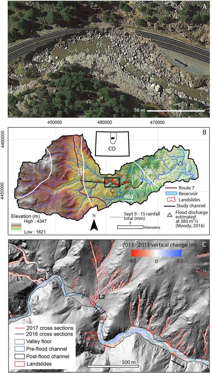
A Example of road damage by channel widening in 2013 flood from neighboring South Saint Vrain catchment, image credit Google Earth, arrow indicates flow direction; (B) North Saint Vrain catchment within the Colorado Front Range, Colorado, USA showing September 9–15 2013 rainfall totals, landslides triggered by the storm (red polygons) and the study reach upstream of Ralph Price Reservoir (adapted from14 and permission received from Geological Society of America to reproduce this). The black box shows the location of the transition reach highlighted in panel C and in Fig. 2 over which the channel transitioned from having very little erosion to dramatic erosion. The inset map shows the location of the catchment in Colorado (CO) with the extent of the storm outlined in dashed black line; (C) DEM of difference of transition reach in which a sudden increase in channel widening occurred downstream of L2 between pre-flood channel (blue polygon) and post-flood channel (black polygon) and showing cross sections used to estimate flood peak discharge along transition reach (black and red lines) (Supplementary Figs. 6 and 7), refer to Supplementary Fig. 2 for more detail on channel elevation change in this transition reach; L1 and L2 refer to key landslides referred to in the text. Pre- and post-flood channel and the valley floor (thin black polygon) were mapped manually, as described in the Methods. Flow in North Saint Vrain Creek is from left to right as indicated by arrow.
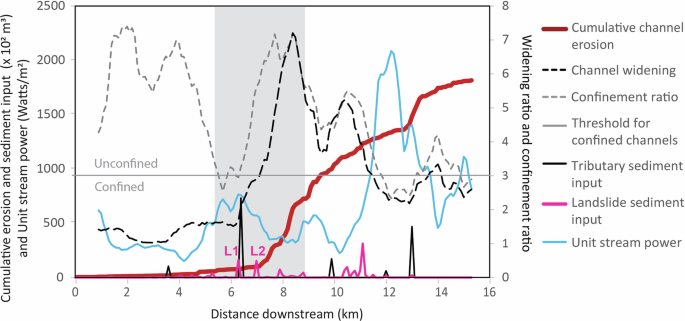
Downstream patterns of cumulative channel erosion (thick red line) and channel width ratio (black dashed line) are shown relative to tributary and landslide sediment inputs (black and pink lines respectively) and modeled stream power (blue line). The confinement ratio is plotted on the secondary y-axis (gray dashed line) along with channel width ratio (black dashed line). A low value of the confinement ratio represents areas that are more confined. The threshold for confined channels as defined by ref. 10 is also shown by solid horizontal gray line. Transition reach shown in Fig. 1C, Fig. 3, and simulated in Fig. 4 is highlighted by the gray-shaded area. L1 and L2 refer to key landslides referred to in the text.
We first attempt to quantify and relate the pattern of channel widening to unit stream power, channel confinement and lateral sediment supply (Fig. 2). We then use field analysis to estimate flood peak discharge and calculate a ratio of flood peak discharge to rainfall-runoff with which to provide an initial test for hypotheses 1 and 2. Finally, we use numerical modeling with a multi-phase flow model to test all three hypotheses concerning landslide-flood interaction. Some methods are further expanded upon in the results sections below and additional detail on methods can be found at the end of the paper in the Methods section.
The study channel as a whole has an average channel width of ~10 m and slope of 0.03 m/m and has cascade, step-pool or riffle-run morphology in cobble to boulder-sized bed sediment. There is discontinuous bedrock exposed along its bed and banks but the channel is predominantly formed in coarse, bouldery alluvium. Montane pine forest is present along hillslopes within the more confined valley reaches, and willow dominates the riparian zones of the less confined valley reaches.
Results
Evidence of landslide-flood interaction from DEM of Difference
We used a DEM of Difference (DoD) produced from pre and post flood LiDAR as detailed by ref. 14. Details of channel change analysis based on the DoD are given in the Methods. The first 7 km of the ~16 km study channel had little channel erosion (~1.4 m3/m) and an average widening rate of 5 m or just half of the average preflood channel width (9.94 m) and a width ratio (i.e. width after/before the flood) was 1.6 (Fig. 2). The valley floor remained largely undisturbed (also refer to37). From around 7 km downstream (i.e. entry point of landslide L2 in Fig. 2), channel erosion (~20.7 m3/m) was much greater and had an average widening of 28 m and a width ratio of 3.76. The flood almost fully occupied the valley floor and so widening was achieved mostly through removal of valley floor sediment, although with some potential evidence of bedrock erosion on outer bends of the channel (e.g., Supplementary Fig. 5). The most rapid transition occurs at 7 km downstream over the 3.5 km transition reach, where channel widening reached 67 m, width ratio reached 9.44, and erosion averaged 38 m3/m. This transition is not explained by peak flood stream power (Fig. 2), as estimated from radar-based rainfall data (see Methods), which increases gradually downstream but does not provide the trigger of the sudden increase in channel width ratio. Whilst channel confinement, calculated as the ratio of valley width to pre flood channel width, constrains channel widening beyond 7 km downstream (Fig. 2 and Supplementary Fig. 3), there is little channel widening for the first 7 km of the channel despite relatively unconstrained channels (i.e., confinement ratio ≥310) along the entirety of the study channel. There are also no obvious variations in channel bank material or riparian vegetation that would explain this increase in channel widening. However, the sudden increase in channel erosion and widening does occur just downstream from three major lateral sediment inputs from two landslides (L1, L2 in Figs. 1C and 2) and a tributary, totaling ~105,000 m3. Further downstream increases in width ratio also correspond to large lateral sediment inputs, but we focus on explaining the largest peak highlighted in Fig. 2. We used a combination of field data and numerical modeling to investigate the potential mechanisms by which landslide-channel interactions may have resulted in the pattern of channel erosion observed. We tested the hypotheses that the pattern of channel erosion generated by the flood was amplified by (1) bulking of the flow by landslide and tributary sediment; (2) damming of the flow by landslide and tributary sediment, and subsequent failure of this dam resulting in an erosive flood surge similar to that observed in debris flows32.
Field evidence of landslide-flood interaction
As an initial test for sediment bulking or surging of the flow that may explain the sudden increase in channel erosion and widening, we calculated the ratio C (field-measured peak discharge/runoff-based peak discharge32). Flood flows can have a range of C values between 0 and 138. Due to conservation of mass, this ratio cannot exceed 1 in the absence of substantial sediment bulking or surge dynamics and can be used as a check on indirect measurements of flood discharge35. A value of C > 1 is diagnostic of bulking of the flow and a value of C > 2 is indicative of surging in the flow, that would provide initial support for hypotheses 1 and 2 respectively. We visited the reach of increased channel erosion in October 2016 and August 2017 to make indirect measurements of flood peak discharge (Qpeak) with which to compare our estimated runoff-based discharge (Qrunoff) (see Methods) and calculate the ratio C.
We used a differential Global Positioning System (GPS) to collect pairs of highwater marks at 23 channel cross sections upstream and downstream from the transition reach (Fig. 1C) in 2016 and 2017 with a vertical and horizontal precision of 0.6 m and 0.4 m, respectively. We identified highwater marks from the 2013 flood based on debris lines on the channel banks and debris trapped in trees. These highwater marks were relatively undisturbed in the 3–4 years since the 2013 flood event given the absence of a larger flood event over this time period16. We used the highwater marks within ArcGIS (Esri, Redlands, California) to extract cross sections from lidar data. Where there is deviation in highwater mark elevations between the left and right banks (i.e. resulting in different reconstructed water levels), we propagate this uncertainty into our estimation of peak discharge cross-section area (Supplementary Figs. 6 and 7). Additionally, we calculated cross-section areas using both pre- and post-flood lidar to account for uncertain channel topography during the flood. We calculated peak discharge in m3 s-1 as
where A is cross-section area in m2 and V is velocity in m s-1. Velocity was calculated using the critical flow method as:
where R is hydraulic radius in m calculated as (R=frac{A}{P}), where P is wetted perimeter in m, g is acceleration due to gravity, and assuming critical flow (i.e., Froude number = 1). The critical flow method has been shown by35 to give values most representative of the average flow conditions during the flood from an ensemble of peak discharge estimation techniques, potentially due to smoothing of the channel bed by sediment infilling during the flood.
Although Qrunoff only slightly increases along the transition reach from about 217 to 218 m3/s, Qpeak shows a rapid increase from 72 m3/s (±5 m3/s) to 468 m3/s (±190 m3/s) over the ~300 m downstream from L2 (Fig. 3C). Therefore, the estimated runoff coefficient, C, also increases from 0.33 ( ± 0.02) to 2.15 ( ± 0.87), with values >2 diagnostic of surge type behavior as can occur in debris flows (Fig. 3C)32.
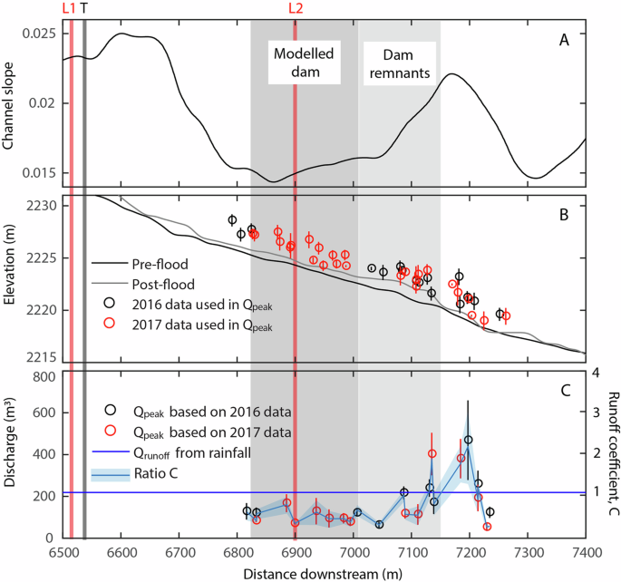
A Channel slope along the transition reach shown in Fig. 2 showing a decrease in channel slope coinciding with modeled dam formation; (B) pre- and post-flood channel profiles in black and gray lines respectively and highwater marks (red and black open circles with error bars) collected at 23 cross sections showing wedge of sediment remaining after the flood downstream from L2; (C) Qpeak calculated from high water marks together with lidar (Figs. S6 and S7 and Table S1) in red and black open circles with error bars and Qrunoff modeled using rainfall data (dark blue line) and ratio of these (C) (lighter blue line with blue shading showing uncertainty). C > 1 is indicative of a dam burst event. Dark gray band shows location of modeled dam that formed around the point of entry of L2 (Fig. 4). Light gray band shows location of remnants of dam observed in the field (Supplementary Fig. 1).
Downstream from the L2 landslide entry, a cobble and boulder rich bar is clearly visible in satellite photos (Supplementary Fig. 1) and was found to have a median grain size of 22 cm (Supplementary Fig. 4). The post-flood channel profile also shows this wedge of sediment (Fig. 3B). We used numerical modeling, detailed below and in Methods, to test the hypothesis that this bar is what remains of a dam that was formed and then removed during the flood (Hypothesis 2). The precise timing of landslides that could have caused a valley damming event is uncertain but previous modeling of landslides in the catchment (including L2) indicates landslides occurred shortly after storm rainfall peaked late in the evening on September 11, with landslides on south facing slopes (including L2) occurring late in the evening of September 11 and landslides on north facing slopes occurring in the early morning of September 1239. Witness accounts also record the first landslides happening at this time in neighboring catchments34,40.
The ratio C calculated based on our field observations supports hypothesis 2 of a dam failure event because the rapid jump in widening at a distinct channel location indicates that a surge of sediment and water similar to a debris flow would be needed to generate erosional widening over a short distance. A dam failure could explain the bank erosion by bulking the flow and generating a positive feedback on bank erosion and channel widening. This has been observed for other dam burst events19, and therefore the dam failure hypothesis may explain the observed profound channel widening of up to 67 m.
Multi-phase modeling of landslide-flood interaction
To further test hypothesis 2 of a dam formation and failure event, we carried out numerical simulations with the computational model r.avaflow (v. 2.4)41 to simulate sediment delivery to the valley floor and its interactions with the fluid flow of North Saint Vrain Creek. The computational model r.avaflow is a freely available deterministic, multi-phase model, which is based on the principles of energy and momentum transfer between liquid and solid phases, extending the use of a Voellmy-type resistance model to multiple phases41,42. Furthermore, r.avaflow has been used to simulate a range of hydro-geomorphic process chains including rock avalanches43, transition of rock avalanches into debris flows44 to glacial lake outburst floods triggered by landslides into lakes45. For fluvial systems, r.avaflow has been validated for glacial debris flow mobility in mountainous river channels46, entrainment of sediment by debris flows in channels47, and channel changes from cascading rockslide-channelized debris flow42. Until recently, it has not been used to simulate landslide-flood interaction29, despite the likely role that sediment supply has in flood dynamics.
For the simulation input, we used the landslides mapped from the DoD for the solid phase and the discharge Qrunoff for the fluid phase. Because the total simulation time is relatively small (900 s in total), the fluid hydrograph has been taken as a constant discharge, corresponding to the peak flow Qrunoff. Because the landslides were mostly formed by coarse sediment (based on in situ observations after the event), the input sediment phase was considered only as coarse (i.e., friction-dominated for the model computations), whereas no input has been used for the fine phase (i.e., inclusive of viscous effects). Although large wood likely played a role in channel widening in this event14, r.avaflow currently does not include this component, but this could be considered in future versions of the model, particularly in the case of hyper-congested flows48. As detailed below, simulations support the formation and removal of a dam downstream of L2, lending support to hypothesis 2. However, it was necessary to perform the simulation in two stages due to a limitation of the model in the version used (2.4), where topography is not updated during the model simulation. In stage (1) dam formation is simulated related to triggering of landslides L1 and L2 and delivery of sediment to the channel and topography is updated to include the dam, and in stage (2) dam removal is simulated using updated topography from stage (1). Boundary conditions and flow hydrographs remain the same for both steps. In the model, landslides have been assumed to be released simultaneously. This had minor effects on the simulations because the delivery time to the valley bottom was different for each individual landslide, and all occurred within 30–45 s from the start of the simulation. Several sets of simulations have been conducted to explore the parameter space, including mobility and erosive parameters (such as drag coefficient and friction), as well as the hydrographs of the main channel and tributary (Supplementary Table 2). Because all parameters are physically based, we used values that are conventionally found in the literature or recommended by the r.avaflow manual49 depending on the type of event.
Figure 4 shows the topographic change within the study area at the end of the simulations for both dam formation (first stage) (Fig. 4a) and dam removal (second stage) (Fig. 4b) superimposed on the observed post-event channel extent. Irrespective of the parameters used for the simulations, the model supports the formation of a large sediment dam in the channel downstream from L2, as well as another smaller dam upstream related to L1 (Fig. 4a). Furthermore, when the topography of the area is updated with the deposition (or erosion) heights from the first simulation stage, the second stage model runs (Fig. 4b) show that substantial erosion occurs, removing the large dam within the simulation time of 900 s. The bulk of the dam is eroded over a period of ~300 s and leads to the erosion and widening of the channel immediately downstream, due to bulking of the flow by sediment. After this time, changes to channel topography was, in comparison, negligible. The final simulated topographic change (Fig. 4c) corresponds well with the observed pattern of erosion from the DoD shown in Figs. 1c and 2. There are some discrepancies between the simulation and observations. For example, the simulated dam occurs closer to the toe of the landslide L2 than the remnants of the dam we observed in the field, which occur ~100 m downstream (Fig. 3). However, these are to be expected considering challenges in replicating spatially explicit two- and three-dimensional landscape evolution in fluvial morphodynamic models50.
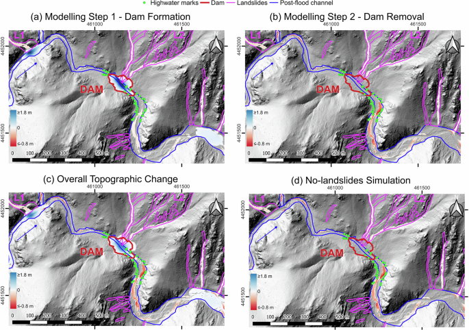
a formation of the sediment dam outlined by red polygon, (b) dam removal with updated topography, (c) the resulting topographic change after both simulations, (d) the results of the simulations with no landslide sediment delivery, highlighting the importance of landslide sediment delivery for simulating observed channel widening. The blue arrow indicates flow direction, whilst the dam extent was mapped for values of deposition ≥0.05 m. Pink polygons show landslides, blue polygon shows post-flood channel and green circles show highwater marks used for calculation of flood discharge (Qpeak) in Fig. 3.
To further test hypothesis 2 that the topographic change of the channel was caused by the formation and then removal of the sediment dam, we performed an additional simulation (Fig. 4d) without landslide sediment input, to evaluate whether the flood flow alone and the sediment it mobilized from upstream to downstream (i.e., not including landslide sediment input) could have caused the channel change. In this scenario, only limited erosion (i.e., <0.10 m) was observed in the main channel downstream from L2 and the extent was substantially smaller than the post-event observations.This is in contrast with the simulations inclusive of landslide input (Fig. 4c), in which the post-event channel extents were much more consistent with the observed changes. The simulated volume of erosion along the channel downstream of the sediment dam is only 518 m3 in the simulation without landslides, compared to 1779 m3 when landslides are included. We therefore conclude that a landslide-dam failure and rapid delivery of sediment best explains the observed geomorphic channel change during the flood. All the numerical simulations involving landslides qualitatively agree on the formation and removal of a dam, whereby the downstream channel widening resulted from bulking of the flow by sediment related to a removal of the debris dam. This lends support to both hypotheses 1 and 2, and the ability of the model to simulate geomorphic change during floods accounting for large lateral sediment supply supports hypothesis 3.
Discussion
Previous studies have documented cycles of hillslope-channel coupling over multi-event timescales with hillslopes delivering sediment to the channel during a rainstorm, for example, and subsequent floods clearing this from the channel system51,52,53. Other studies have documented the occurrence of landslide-dams and the erosive power of dam burst floods, whether landslide induced or otherwise19,54. Here, we have documented with a combination of detailed field data analysis and numerical modeling how landslide-delivered sediment may interact with the main channel during an individual flood through formation and failure of a dam and bulking of the flow by sediment i.e. hypothesis 2. In agreement with prior studies, we observed that landslides delivering sediment into a fluvial channel led to channel widening23,24,25,26,27,28.
Here we outline the observed and simulated process-chain with the following stages. In Stage 1, landslides triggered by heavy rainfall deliver sediment to the flood flow and temporarily dam the channel. In Stage 2, the flood starts to gradually remove the dam, bulking the flow with sediment and causing it to erode channel banks and bed downstream. In Stage 3, the flow continues to be loaded with sediment from the dam and from bank erosion causing further erosion of outer banks, although remnants of the dam remain. Although it is likely that large wood played a role in the pattern of channel widening14 as observed in other catchments55, modeling indicates that sediment delivered by landslides to the flood flow is crucial for explaining the substantial channel widening observed in this event (Fig. 4c,d). We have focused here on the damming and erosion related to the larger landslide L2, although we note that farther upstream landslide L1 also forms a small dam at its toe in the model and probably explains the channel widening of the opposite bank of the river at that location (Fig. 4b). We also note the correlation between channel widening and landslides further down the study channel in Fig. 2, e.g. at 11 km downstream. This reach was not included in simulations due to constraints in computational resources, hence it is unclear whether a further dam may have developed and failed or whether simple bulking of the flow by sediment could have produced channel widening (i.e. hypothesis 1).
We have focused on landslide sediment delivery directly into the study channel but sediment input from tributaries may result in similar effects. For example, at ~13 km downstream a tributary delivered ~5 ×10⁴ m3 of sediment (predominantly from landslides along the tributary) potentially damming and/or bulking the flow and resulting in the peak in channel widening just downstream. We suspect that similar landslide-channel interactions may be responsible for higher than expected peak discharge relative to rainfall runoff in other Colorado Front Range catchments flooded in 201335. Furthermore, such landslide-channel interactions may be relevant for understanding and predicting channel widening and erosion during floods in other mountainous regions of the world. Given that extreme rainfall and associated landslides and flooding are expected to increase in a warmer climate31, and that extreme rainfall can be more important in generating landslides than earthquakes, even in places that are tectonically active56,57,58, such landslide-flood interactions will be increasingly important to account for. We have also demonstrated the role of multiphase models such as r.avaflow in simulation of flood dynamics in cases of high lateral sediment supply (i.e. hypothesis 3) and recommend that these are further tested for more accurate modeling of flood hazard in catchments where floods typically coincide with high sediment supply29.
Methods
Channel change analysis
The mapping of pre- and post-flood channel widths and valley floor width and calculation of channel widening and erosion is detailed in Supplementary Information. Channel erosion was calculated from pre- and post-flood light detection and ranging (lidar) elevation data detailed in14. Details on calculation of channel erosion and widening ratio were not provided in ref. 14 and so are provided here. A channel centerline was extracted in TopoToolbox 259 from the pre-flood lidar. Points were extracted from this every 20 m, and Thiessen polygons were created around these points (Supplementary Fig. 2). These polygons were clipped into pre- and post-flood channel widths and valley width based on manually mapped extents of these features (Supplementary Fig. 2). Valley width was mapped as the floodplain and any terrace remnants60, although ideally would be mapped using automated tools60 that were less available at the time this analysis was conducted. Channel widening ratio calculated as the ratio of post to pre channel width61. Eroded volume was calculated in each polygon using the budgeting tools in Geomorphic Change Detection62 and was integrated downstream to produce the pattern of cumulative erosion in Fig. 2. Channel confinement was calculated as the ratio of valley width to pre-flood channel width following10.
Runoff-based peak discharge (Qrunoff) and stream power estimation
We estimated flood peak discharge (Qrunoff) with daily National Centers for Environmental Information radar data routed with a 10 m digital elevation model (DEM) in Topotoolbox259. We extracted the drainage network using standard flow-routing algorithms and applied a drainage area threshold of 1 km2 to extract the stream network61. The position of the stream network was validated against the lidar DEM and showed good visual agreement. We used daily rainfall data from 11 September 2013, on the basis that the main flood peak occurred late on this day once soils were saturated and in response to an increase in rainfall intensity towards the end of the day on 11 September33,35. This method assumes steady uniform runoff and zero infiltration or storage, which is a reasonable assumption based on the inference that soils became saturated on this day. Despite the coarse nature of rainfall data and the simplistic nature of our runoff modeling, the modeled discharge at the catchment outlet (682 m3/s) is in the same order of magnitude as the indirect peak discharge measurement of 385 ± 80 m3/s35. Notably the indirect peak discharge estimate was not measured until March and after some of the left bank high water marks had been destroyed by blasting at the mouth of the North Saint Vrain canyon for flood repair work on U.S. Highway 3635, which may reduce reliability of this estimate. The overestimation of our modeled discharge compared to this field estimate is in line with assumptions of zero infiltration or storage and gives us a reasonable approximation of discharge and therefore stream power along the North Saint Vrain Creek with which to compare against the pattern of observed channel widening. We calculated unit stream power for every 100 m reach as: (omega =gamma {QS}/w) where (omega) is unit stream power (W/m2), Q is discharge (m3/s), S is channel slope (m/m), w is pre-flood channel width (m) and (gamma) is the unit weight of water (kg/m3)
Numerical simulations using r.avaflow
The freely available software r.avaflow is a deterministic model based on the physics of interactions between solid and fluid phases41. The model has been used to simulate topographic changes of the valley floor due to sediment delivery from landslides42,63, debris flow erosion47, and more recently for the Chamoli disaster in the Indian Himalaya44. The main principles of the model are based on the Voellmy-type approach41,42, whereby the three phases (i.e., solid, fine, and liquid) interact with each other by momentum balance and energy conservation principles. Input is provided by an elevation map based on the DEM of the study area. For this paper, the DEM resolution was 2 m by 2 m. The model also requires a map (with the same resolution as the DEM) where it is indicated a depth of release (i.e., the depth of material that will initiate motion) for each of the three phases, to simulate the initiation of landsliding. Because the landslides were mostly debris-flow type of coarse size, only solid and liquid phases have been included as release depths, whilst no input has been used for the fine phase. This is in contrast to a similar study in the Philippines where simulation of geomorphic change during a major flood required both coarse and fine sediment phases29. This means that the model only assumed frictional forces between phases. Solid release corresponded to the areas (manually mapped from available satellite imagery) from which landslides originated and their depths extracted by the DEM of difference (DoD) at the landslide release area. For the liquid phase, a constant value of 0.20 m (representative as a fraction of the total average landslide volume) was provided in correspondence of the landslide areas (i.e., on the same cells where solid release was used as input) to account for the soil saturation estimation at the time of the event. In addition, a flow input at the upstream boundary condition has been applied to both main channel and tributaries by using the estimated velocity V. The model also requires a map for the maximum erodible areas for each phase and associated elevations. In this case, the mapping was provided by the DoD and corresponded to the areas of run-out and channel change observed post-event and was used for both solid and liquid phases. The model also requires the definition of several parameters, notably the internal friction and the basal friction (i.e., the friction between the landslide and ground). Variables that have been kept constant in all tests were: the material densities (2700 kg m–3 and 1000 kg m–3 for solid and fluid phase respectively), the tributary hydrograph (discharge Qrunoff) and the friction coefficients, as suggested by the r.avaflow manual for these types of soil, between phases. The main variables that have been changed across the five different tests are displayed in Supplementary Table 2. These were tested to fully represent the spectrum of key physical quantities in the landslide-channel interactions and confirm that the dam formation and its subsequent failure was always observed in the simulations, irrespective of the variation of input parameters. The simulations shown in Fig. 4 were based on the parameters employed in Test 1, which has served as pilot test for the other sets of tests.
Authors have obtained written consent to publish images in Supplementary Information.


Responses