Landslides induced by the 2023 Jishishan Ms6.2 earthquake (NW China): spatial distribution characteristics and implication for the seismogenic fault
Introduction
Strong earthquakes usually cause great damage to the geological environment1,2. In addition, large numbers of secondary geological hazards are induced by earthquakes in high mountain and valley areas3,4. These secondary geological hazards can also cause non-negligible casualties and losses5,6,7. To reduce casualties and losses caused by coseismic landslides, researchers have conducted systematic and comprehensive studies in multiple directions, including triggering mechanisms8,9, database establishment10,11,12,13, spatial distribution patterns14,15, risk assessment16,17, monitoring and early warning18,19, and metric analysis20,21.
These studies not only provide a solid scientific foundation for understanding coseismic landslides but also offer crucial theoretical support for mitigating the impacts of coseismic landslides and formulating effective hazard prevention and control measures. For example, through in-depth research on the triggering mechanisms and spatial distribution patterns of coseismic landslides, scientists can more accurately predict high-risk areas for landslides and propose targeted hazard prevention and mitigation strategies22,23. Moreover, the findings from risk assessment and monitoring and early warning research have been widely applied in several earthquake-prone regions, providing valuable references for local governments and communities in developing emergency response plans24,25. However, the increasing speed and impact of climate change, exacerbated by global warming, along with more frequent human activities, have made the risk of geological hazards more complex and unpredictable26,27,28. Despite significant progress in research, the risk of geological hazards remains high due to the complexity and variability of seismic activity, especially in tectonically active regions, posing ongoing challenges to hazard prevention and mitigation efforts.
The Tibetan Plateau region in western China is characterized by intense tectonic activity and frequent seismic events. These events often trigger a large number of coseismic landslides, posing long-term threats. Notable examples include the 2008 Ms 8.0 Wenchuan earthquake29,30,31, the 2013 Ms 7.0 Lushan earthquake32,33, the 2013 Minxian Ms 6.6 earthquake34,35, the 2014 Ms 6.5 Ludian earthquake36,37,38, the 2017 Ms 7.0 Jiuzhaigou earthquake10,39,40, the 2022 Ms 6.8 Luding earthquake41,42,43.
On December 18, 2023, a magnitude 6.2 earthquake struck Liugou Township, Jishishan district, Gansu Province (35.70°N, 102.79°E) (China Earthquake Networks Center, http://www.ceic.ac.cn). The epicenter was located just 8 km from Jishishan County, with a focal depth of 10 km. The maximum intensity of the earthquake reached VIII (China seismic intensity scale), with the isoseismal long axis oriented in an NNW direction, measuring 124 km in length and 85 km in width. The area of the VII intensity zone covered 1514 km2. This earthquake is the strongest recorded in the region’s history, resulting in significant casualties and property damage, and attracting widespread attention both domestically and internationally. These studies include field investigations44,45,46, emergency coseismic landslides identification47, preliminary analysis and comparison of coseismic landslides48,49, and surface deformation analysis50,51. Despite this progress, there are still areas that need to be further strengthened, especially in terms of the accuracy and completeness of the available data, as many preliminary studies prioritize rapid analyses over detailed spatial patterns. To address these gaps, this study aims to build a comprehensive database of coseismic landslides by comparing and interpreting pre- and post-earthquake remote sensing imagery. This study will incorporate relevant environmental influences to deepen the understanding of landslide distribution patterns. We also hope that the results of the study will support a more accurate identification of seismogenic faults.
Geological background of the study area
The Jishishan region is located in the southeastern part of Qinghai Province, China, and is part of the eastern extension of the Qilian Mountains (Fig. 1a). The region belongs to the Qaidam-Qilian block, characterized by basin-mountain tectonic features under a compressional environment, making it a region of significant tectonic deformation and frequent strong earthquakes in the northern plateau52. According to statistics, there have been 20 earthquakes with a magnitude of 7 or above within the boundary zone of the Qaidam-Qilian active block. Among these, major earthquakes include the 1654 Tianshui earthquake, the 1920 Haiyuan earthquake, the 1927 Gulang earthquake, and the 2001 Kunlun Mountain earthquake (Fig. 1b). The fragile geological structure of the area, as evidenced by the remains of many large ancient landslides53, can be largely attributed to frequent earthquakes. Earthquakes have repeatedly shaken the ground, weakening the integrity of rock formations and destabilizing slopes, thus facilitating the occurrence of landslides over time.
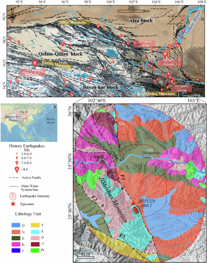
a Topographic map of China and neighboring areas. b Seismotectonic setting of the northern part of the Qinghai-Tibet Plateau and position of the study area. c Simplified geological map of the study area. Codes of the lithology units are the same as in Table 1. Seismic data from the National Earthquake Data Center (https://data.earthquake.cn/), Geologic data from Zuo et al.56.
This study focuses on the area within the seismic intensity VII of the 2023 Jishishan Ms 6.2 earthquake. The study area is dominated by a major fault zone composed of two primary faults with opposite dips, identified as F1 and F2 in Fig. 1c. These faults are referred to in the literature as the East Jishishan Fault and the Western Jishishan Fault54. Fault F3, connected to F2, is the Linxia South brittle thrust fault zone, which also primarily exhibits thrust faulting and forms the boundary between the Jishishan uplift and the surrounding basin. Additionally, several smaller branch faults are distributed in the northern part of the study area, gradually converging from NW to SE towards the main fault zone of the East Jishishan Fault. The study area exhibits a west-to-east transition of geomorphological features, including mountain ranges shaped by tectonic erosion processes, eroded and denuded low hills, and river valley plains. The Yellow River flows from west to east through the study area, making the regional drainage system predominantly composed of tributaries of the Yellow River. The oldest exposed strata in the region are Paleoproterozoic intrusive rocks, with Cretaceous, Neogene, and Quaternary strata widely distributed across the area.
Data and research methods
In this study, landslide data (“landslides” refer to all forms of mass movements in a broad sense) were obtained through the interpretation of multi-temporal optical remote sensing images. The image data were obtained from the PlanetScope multispectral data satellite with a spatial resolution of 3 m. The selected periods include October-November 2023 and January-March 202455. We selected relevant factors to analyze their potential influence on the spatial distribution of landslides, including topography, geology, and hydrological environment. DEM data were sourced from the Copernicus Digital Elevation Model (COP-DEM) released by the European Space Agency, with a resolution of 30 m. Based on this data and using a GIS platform, topographic factors were derived (elevation, slope, aspect and terrain position). Geological maps were obtained from the 1:250,000 digital geological map of China released by the China Geological Survey56, from which lithology, yield points, and fault data were extracted. Hydrological data were sourced from the 1:1,000,000 basic geographic information dataset (2021) released by the Ministry of Natural Resources (https://www.webmap.cn/). The Peak Ground Acceleration (PGA) data were obtained from open-access warning station data57 and interpolated using the empirical Bayesian Kriging method. NDVI data were sourced from the 2022 30 m maximum NDVI dataset released by the National Ecological Science Data Center (http://www.nesdc.org.cn/), as the 2023 data had not yet been published.
Results
Coseismic landslide database
Following the earthquake, we promptly conducted field investigations and carried out a preliminary survey and documentation of coseismic landslides within the affected area. Figure 2 illustrates several typical coseismic landslides observed during these investigations. The findings from these field surveys were subsequently used in our research to compare with remote sensing imagery, helping to enhance the accuracy of our interpretation. In our study area, the majority of landslides are indeed shallow disrupted landslides (See for e.g., Figure 2), with only a few exceptions exhibiting characteristics of large-scale liquefied landslide-debris flows (e.g., Fig. 3c-2). Given the relatively uniform landslide type, we did not include landslide type as a separate variable in our subsequent analysis, instead focusing on the overall characteristics of landslides.
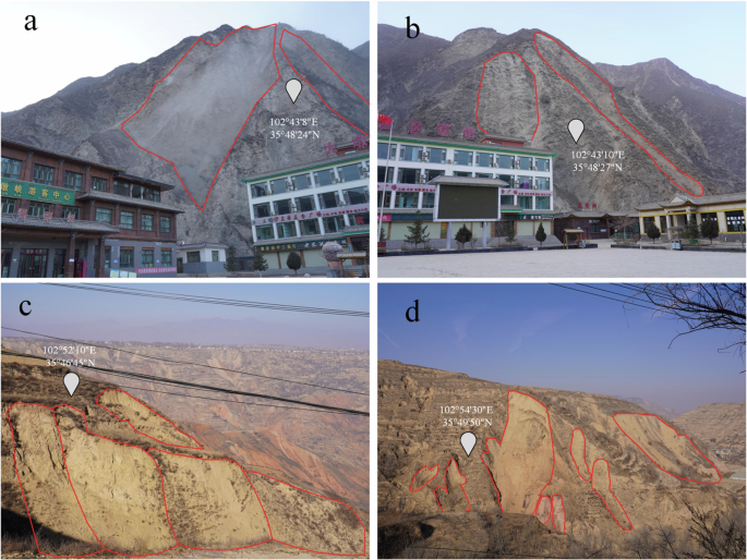
a, b show landslides near houses with significant elevation differences. c, d show landslides densely distributed on the nearby mountain.
The typical landslides have been highlighted with red lines in the images. The location of each image is noted with blue markings and text.
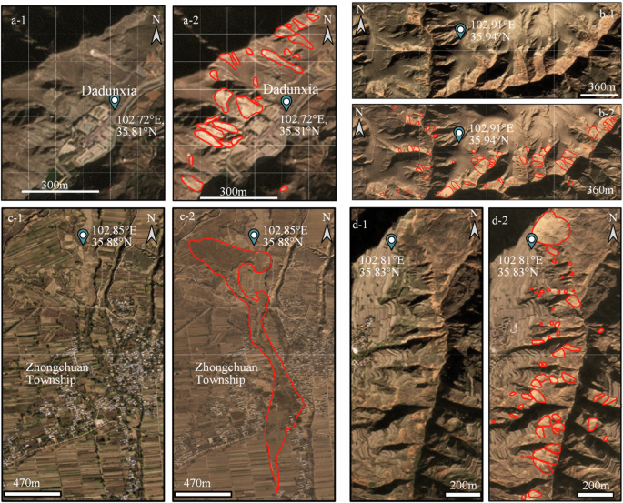
By comparing pre- and post-earthquake remote sensing images, the characteristics of landslides triggered by the earthquake can be visually identified58,59. Figure 3 presents several areas with distinct landslide features. Figures 3a-1 and 3a-2 are located on the western side of the Daduxia area, corresponding to the same location as Fig. 2a, b. Figures 3b-1 and 3b-2 are ~1 km northeast of Minzhu Village in Zhongchuan Township. Figures 3c-1 and 3c-2 are situated in Zhongchuan Township, representing a typical liquefaction-induced landslide-mudflow. The landslide source area is located on the loess platform of the third terrace of the Yellow River, with 0.48 km2 interpreted impact area60. Figures 3d-1 and 3d-2 are from the Qijiashan region, across from the Lajia Ruins.
Through image interpretation, this study identified 2643 landslides within the study area. The spatial distribution of these landslides was analyzed using point density (Fig. 4a) and area density methods (Fig. 4b). Both analyses reveal high-density landslide zones concentrated in the central, northeastern, and southeastern regions of the study area. These zones align geographically with primarily residential areas. Conversely, the mountainous canyon regions in the western part of the study area exhibit lower landslide density.
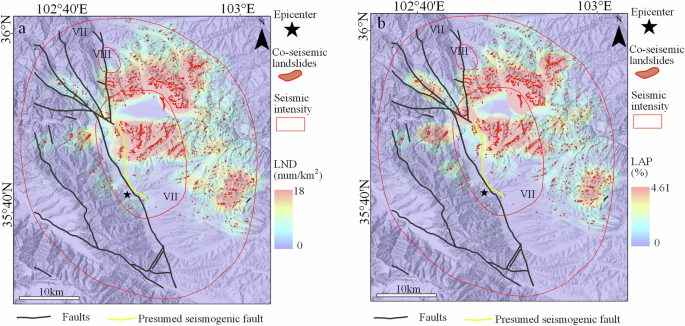
a Map of landslide distribution and point density. b Map of landslide distribution and area density.
Figure 5a presents the logarithmic fit between landslide area and quantity ratio, with the horizontal axis representing the logarithm of landslide area and the vertical axis showing the proportion of landslides exceeding each corresponding scale. The Jishishan coseismic landslides span a total area of 4.36 km2, with the largest individual landslide covering approximately 481,950 m2, and an average landslide size of 1645.7 m2. Notably, 59% of the landslides (1557 events) are smaller than 1000 m2, indicating a generally moderate landslide scale, with only a few exceptionally large occurrences. Figure 5b provides a comparative analysis of recent seismic events of similar magnitude in western China, juxtaposed with the Jishishan earthquake61,62,63,64. The epicenters of the earthquakes involved in Fig. 5b are shown in Supplementary Fig. 1. All these events occurred in western China, near or within the Tibetan Plateau region. The 2022 Ms 6.0 Maerkang earthquake, the 2022 Ms 6.8 Luding earthquake, and the 2019 Ms 6.0 Changning earthquake all took place in western Sichuan Province, a region influenced by multiple fault zones. The 2019 Ms 6.9 Milin earthquake occurred in Milin County, Tibet, along the Yarlung Zangbo fault zone on the southeastern edge of the Tibetan Plateau. These areas experience frequent seismic activity due to the active tectonics resulting from the collision between the Indian Plate and the Eurasian Plate. The results indicate that the overall scale of the coseismic landslides in the Jishishan earthquake is similar to that of the Maerkang earthquake but smaller than that of the Luding earthquake.
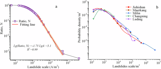
a Area-frequency plot of the Jishishan earthquake; b comparative analysis of landslide scales triggered by earthquakes of similar magnitude.
Relationship analysis of influencing factors
Previous studies have shown that the occurrence of coseismic landslides is influenced by both seismic factors and predisposing environmental factors. Seismic factors, such as the energy released during the earthquake and the intensity of ground shaking, significantly influence the extent of damage to rock and soil materials. Meanwhile, predisposing environmental factors determine the stability and susceptibility of the rock and soil, significantly influencing the extent of earthquake damage. For example, factors such as topography and geomorphology65,66, stratigraphy and lithology67,68,69, fault structures41,70, and vegetation cover71,72 play significant roles. When seismic factors and predisposing environmental factors reach certain critical conditions or form specific combinations, coseismic landslides may be triggered. Selecting relevant influencing factors is essential to accurately analyze the spatial distribution of coseismic landslides in real earthquake events. In this study, we considered a comprehensive set of topographic, geological, hydrological, and seismic factors, initially screening 13 environmental variables. Using correlation analysis and the Pearson coefficient as the selection criterion, we identified 9 significant factors (Supplementary Fig. 2): elevation, slope, aspect, terrain position, stratum, slope structure, distance to rivers, NDVI, and PGA.
Topographic factors
Elevation, as a key topographic factor, significantly influences geological conditions, precipitation and snowfall patterns, climate, vegetation cover, and seismic wave propagation. Higher-altitude areas, for instance, tend to feature rugged terrain and fractured rock formations. Variations in elevation correlate with distinct climatic conditions, including differences in precipitation type (rain vs. snow), amount, and temperature, which in turn affect vegetation types and density. These interconnected factors collectively shape landslide distribution patterns, with similar elevation ranges within a region likely exhibiting comparable impacts on landslide occurrence.
Figure 6a illustrates the overall elevation distribution in the study area, showing a trend of higher elevations in the west and lower elevations in the east, with an elevation range between 1700 to 4636 m. The highest elevation where landslides occurred is 3478 m. Landslides are sparsely distributed in the high-altitude southwestern region of Jishishan Mountain and are more prevalent in the central and eastern hilly areas of the study area. Figure 6c provides statistics on landslide distribution across different elevation intervals. It includes data on landslide area, landslide number, and the Landslide Area Percentage (LAP) for each interval. Consistent with the phenomenon reflected in Fig. 6a, the landslides triggered by this earthquake are mainly distributed between 1700 and 2300 elevation. Notably, in the 1700–2000 m interval, the LAP is the highest at 0.72%. In the 2000–2300 m interval, there are 1675 landslides (accounting for 63.4% of the total number of landslides) and a landslide area of 2.36 km2 (accounting for 54.2% of the total landslide area), making this the interval with the highest proportion of both the number and area of landslides.
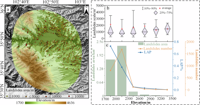
a Elevation distribution in the study area. b Landslide scale within each interval. c Landslide statistics within each interval.
Given the presence of a few extremely large-scale individual landslides, the trend of the distribution pattern might be affected. To account for this, a box plot for the scale of individual landslides in each elevation interval was created, as shown in Fig. 6b. In this study, the term ‘landslide scale’ refers to the area of individual landslides, distinguishing it from the total landslide area within each interval. In the box plot, the box represents the interquartile range (25–75%) of the landslide scale, with the horizontal line inside marking the median. The whiskers extend from the 10% to 90% range, reducing the influence of extreme outliers. Results indicate minimal variation in the interquartile range across elevation intervals, while the median gradually increases with elevation. This trend suggests that larger landslides are more likely to occur at higher elevations.
Slope reflects the steepness and stability of the terrain. Steeper slopes are more likely to cause the instability of rock and soil masses, increasing coseismic landslides. Additionally, slope and elevation differences can affect the scale and impact range of coseismic landslides. Figure 7a shows that the highest slope in the study area reaches 72°, and the overall distribution aligns with the direction of the mountain ranges. Figure 7c displays statistical results showing that both the number and area of coseismic landslides initially increase and then decrease with a rising slope angle. In the 20–30° slope range, there are 888 landslides (33.6%) covering a total area of 1.15 km2 (26.4%). In the 30–40° range, 677 landslides (25.6%) occupy an area of 1.18 km2 (27.1%), indicating these two intervals as the primary concentration zones for coseismic landslides. Additionally, Landslide Area Percentage (LAP) peaks at 1.26% in the 50–60° interval, suggesting that steeper slopes exhibit a higher landslide proportion. Figure 7b corroborates this pattern, as higher slope intervals (excluding 0–10°) show a progressively elevated box plot position and increased average values. Thus, coseismic landslides most frequently occur within the 20–40° slope range, with individual landslide scales increasing alongside the slope.
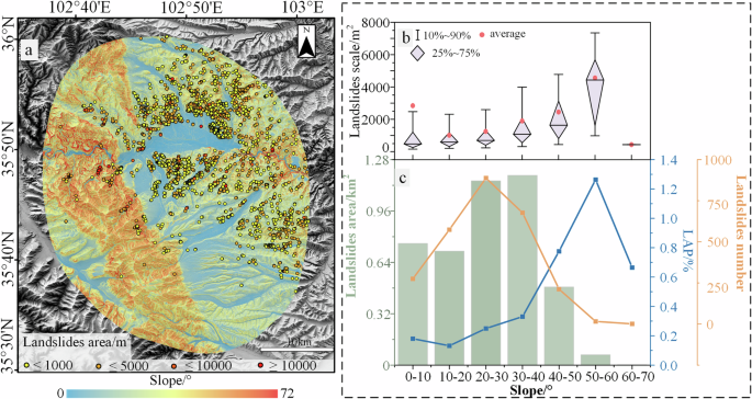
a Slope distribution in the study area. b Landslide scale within each interval. c Landslide statistics within each interval.
Generally speaking, the slope aspect is related to the propagation direction of seismic waves. If the slope aspect aligns or closely matches the direction of seismic wave propagation, the amplification effect of the seismic motion will be more pronounced, resulting in greater PGA and duration73,74. Additionally, different slope aspects receive varying amounts of sunlight, which can lead to differences in soil properties and vegetation cover75. In this study, the north is designated as 0°/360°, with clockwise rotation defined as positive, dividing the slope aspect into eight intervals (Fig. 8a). Analysis results in Fig. 8b–d reveal a consistent distribution pattern, with the SE and S aspects showing a clear predominance in landslide count, total landslide area, and LAP. This directional preference aligns with the orientation of the seismic intensity’s long axis.
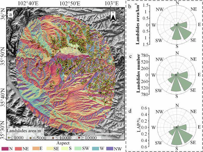
a Distribution of slope aspect in the study area. b–d Landslide area, number, and LAP statistics in different slope aspect intervals.
Slope position, also referred to as the Topographic Position Index (TPI), measures the relative height of a location compared to its surrounding terrain, characterizing topographic features. Figure 9a show the TPI distribution across the study area. The slope was categorized into five intervals, ranging from valleys to ridges, with equal spacing: lower slope (−1 to −0.6), mid-lower slope (−10.6 to −0.2), middle slope (−0.2 to 0.2), mid-upper slope (0.2–0.4), and upper slope (0.4 to 1). As shown in Fig. 9c, landslide occurrence and area are concentrated predominantly in the middle and mid-lower slope intervals. The middle slope interval contains 1217 landslides (46%), covering an area of 2.13 km2 (48.9%). Notably, the LAP in the lower slope interval reaches a maximum of 0.65%, indicating a higher probability of landslide occurrence in this zone. This may be due to water accumulation at slope bases, increasing moisture content. In the study area, the strength of loess is notably reduced when saturated, which makes it more prone to liquefaction under seismic activity, thus elevating landslide susceptibility. Figure 9b shows that the box plot for the middle slope interval has higher values across the box position, whiskers, and average, while other intervals show less variation in landslide scale. Overall, coseismic landslides are predominantly distributed in the middle and lower slope intervals.
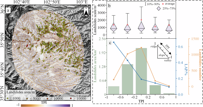
a TPI distribution in the study area. b Landslide scale within each interval. c Landslide statistics within each interval.
Engineering geology and hydrological factors
Considering only the superficial lithology for landslide triggering is insufficient. Additionally, conducting an engineering geological strength assessment for each landslide might present practical challenges. Furthermore, even with the same lithology, factors such as formation time, burial depth, and the pressure exerted by overlying layers can influence engineering geological characteristics. Given this, the study selected the geological map-provided stratums of different formations in the study area as one of the influencing factors. Each Stratum category includes multiple lithologies, and formations of similar ages tend to have relatively similar soil and rock combinations (Table 1).
Fig. 10a shows the distribution of coseismic landslides and stratum in the study area. In the southwestern part of the study area, specifically the Jishishan region, the stratum is mainly composed of Silurian and Ordovician. The eastern part of the study area features extensive outcrops of Neogene sedimentary rocks and Quaternary deposits, including loess. In the central part of the study area, around the Yellow River basin, the stratum is predominantly Paleogene. According to Fig. 10b, in the stratums from the Cambrian to the Silurian, the box and whisker plot ranges are slightly higher than in other zones, indicating that landslides in these zones tend to be larger in scale, corresponding to the mountainous canyon areas in the eastern part of the study area. The statistical results in Fig. 10c show that most landslides are concentrated in the Paleogene and Neogene stratum. Among them, 1080 landslides (40.86%) with a total area of 2.19 km2 (50.22%) are distributed within the Paleogene zone, and 1052 landslides (39.8%) with a total area of 1.28 km2 (29.36%) are found in the Neogene zone.
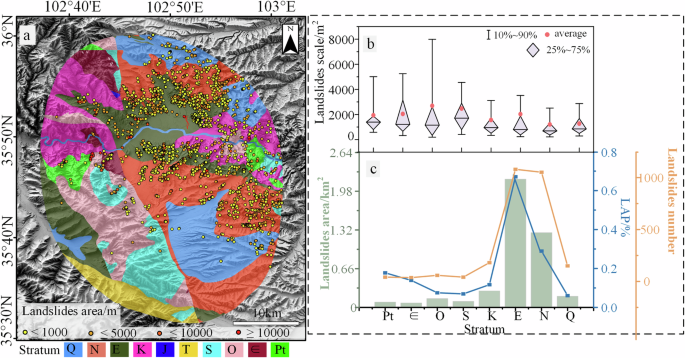
a stratum distribution in the study area (b) Landslide scale within each interval. c Landslide statistics within each interval.
The stratigraphy exposed in the study area exhibits primary layered characteristics, with the primary stratified structural planes of the strata serving as the main controlling structural planes for landslides. The slope aspect determines the free-face conditions of the landslide, making the relationship between the dip direction of the strata and the slope aspect, as well as the dip angle of the strata and the slope angle, an influential factor in triggering coseismic landslides. This study uses slope structure types to reflect the relationship between the primary layered structural planes and the slopes. By utilizing occurrence data points from regional geological maps, a dip direction raster was generated. By combining this with the previously obtained aspect raster, the difference between the bedrock dip direction and the slope aspect was calculated and then reclassified into different intervals: consequence slope (0–30°), inclined slope (30–60°), transverse slope (60–120°), reverse inclined slope (120–150°), and reverse slope (150–180°).
Figure 11a shows the distribution of slope structures in the study area. In Fig. 11b, the height distribution of the box plots in each interval is similar. In Fig. 11c, the transverse slope interval contains 1007 landslides (38.1%), covering an area of 1.8 km2 (41.28%), both of which are the highest values among the intervals. The inclined slope interval ranks second in terms of landslide quantity and area, with a LAP of 0.38%, the highest among all intervals. We believe that landslides are more favorably distributed in these two intervals. In the inclined slope, the strata dip angle is similar to the slope angle, and the inclination direction of the strata facilitates the occurrence of sliding. During an earthquake, the combined effects of the strata’s weight and seismic motion easily cause the strata to slide along the dip angle. In the transverse slope, the dip direction of the strata intersects with the slope aspect, leading to concentrated stress. This also has some correlation with the larger area proportion of transverse slopes within the study area.
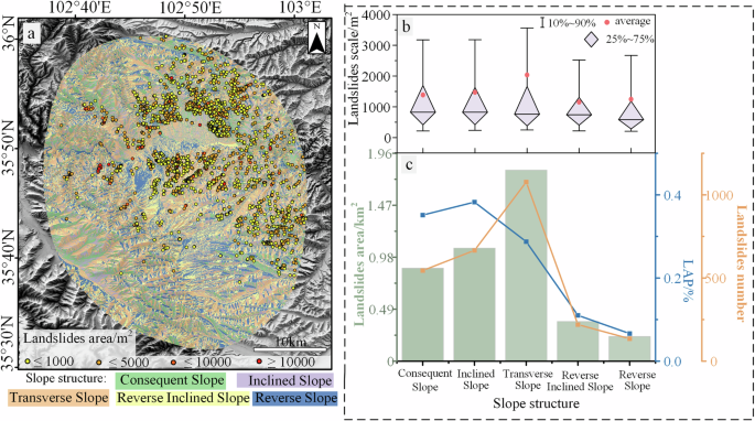
a Slope structures distribution in the study area. b Landslide scale within each interval. c Landslide statistics within each interval.
The distance to rivers reflects the hydrological conditions of the slope. The erosion and scouring effects of water systems can reduce the stability of slopes and increase the likelihood of coseismic landslides. Given the extensive distribution of rivers, most areas within the study region are less than 2 km away from a river (Fig. 12a). In Fig. 12c, both the number and area of landslides decrease as the distance to the river increases. Within 400 meters of the river, there are 1184 landslides (44.8%) with a total area of 2.06 km2 (47.24%). The LAP suddenly increases beyond 2 km from the river. This phenomenon is explained in Fig. 12b, where the box plot position rises beyond 2 km, with the whisker height and mean value also increasing. This indicates that while the total number of landslides is small in this interval, the overall scale is larger. Additionally, since the area in this interval is much smaller than others, this results in a sudden increase in LAP. Because these landslides are farther from the river, they are less influenced by it. Therefore, in terms of the relationship between coseismic landslide distribution and proximity to rivers, it can still be concluded that areas closer to rivers are more favorable for landslide distribution.
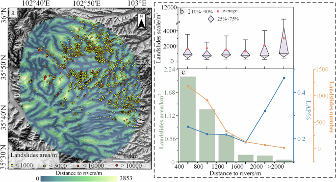
a River distribution in the study area. b Landslide scale within each interval. c Landslide statistics within each interval.
The Normalized Difference Vegetation Index (NDVI) is an indicator used to measure vegetation cover and health. Vegetation on slopes can increase soil shear strength through the reinforcement provided by root structures, thereby enhancing slope stability. High NDVI values indicate good vegetation cover, while low NDVI values indicate sparse or degraded vegetation. In Fig. 13a, NDVI values are higher in the southwestern part of the study area and lower in the central and eastern regions. In Fig. 13c, within the NDVI interval of 0.4–0.6, there are 1507 landslides (57.21%) with a total area of 2.02 km2 (46.33%), both representing the maximum values. The highest LAP is found in the NDVI interval of 0.2–0.4, at 0.71%. Figure 13b shows that in the NDVI interval of 0–0.2, the box plot height is the highest; however, this interval contains only 6 landslides, which are relatively large in scale. Comprehensive analysis suggests that coseismic landslides are most favorably distributed within the NDVI interval of 0.2–0.6. This finding aligns with the observation that areas with low NDVI values, which lack the reinforcing effects of vegetation, are more prone to instability under seismic motion, making landslides more likely to occur.
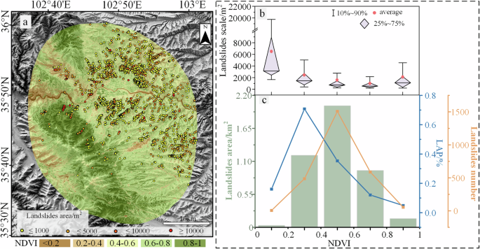
a NDVI distribution in the study area. b Landslide scale within each interval. c Landslide statistics within each interval.
Seismic factor
In terms of seismic factors, we have determined to use PGA as a reflection of seismic impact. In Fig. 14a, the maximum PGA is 0.9 g, with a decreasing trend from the central part of the study area toward the periphery. In Fig. 14b, within the interval of PGA less than 0.75 g, the box plot positions for each interval show little difference as PGA increases, but the average size of landslides tends to increase. Figure 14c shows that within the 0.45–0.6 g PGA interval, there are 1172 landslides (44.34%) with a total area of 2.18 km2 (50%), both representing the maximum values. In the 0.75–0.9 g PGA interval, the LAP is highest, at 0.57%, indicating that within the interval where PGA is greater than 0.75 g, the area is smaller, and small-scale landslides are densely distributed. Therefore, landslides are most favorably distributed within the 0.45–0.6 g PGA interval.
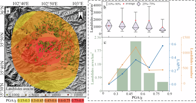
a PGA distribution in the study area. b Landslide scale within each interval. c Landslide statistics within each interval.
Relative importance of factors
In analyzing the relative importance of the factors influencing landslide distribution, we aimed to explore the weight differences of various environmental factors. To achieve this, we carefully selected 2643 sample points from both landslide-affected and non-affected areas to construct our dataset and employed the XGBoost model for analysis. The XGBoost model, renowned for its powerful ensemble learning capabilities, chooses splitting nodes based on the contribution of each feature to classification or regression tasks during training. The F_score serves as a key indicator that measures the frequency with which each feature is selected as a splitting node. (Fig. 15)
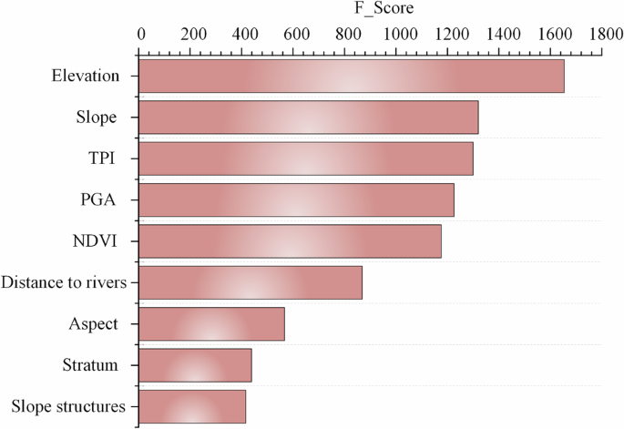
Relative importance of factors.
Our analysis identified key factors influencing landslide occurrence as elevation, slope, TPI, and PGA. Elevation is closely linked to geological conditions, climate, vegetation cover, and seismic wave propagation characteristics. The distribution of landslides varies significantly across different elevation ranges, with a noticeable concentration occurring between 1700 and 2300 meters. Furthermore, larger-scale landslides are more likely to occur at higher elevations, indicating the foundational role of elevation in the initiation and development of landslides.
The slope is another critical factor reflecting the steepness and stability of the terrain, with the range of 20–40° identified as a high-frequency zone for landslides. As the slope increases, the scale of individual landslides also tends to grow, underscoring its essential role in triggering landslides. TPI, which measures the relative height of the terrain, reveals the significant impact of micro-topographic features on landslide distribution, with landslides predominantly occurring in mid-lower slope positions where the topographic conditions favor their formation. Finally, PGA directly correlates with seismic shaking and its potential to trigger landslides; we observed the densest landslide distribution within the 0.45–0.6 g range, indicating that seismic motion within this intensity range has a significant impact on landslide triggering in the study area.
Discussion
Regarding this earthquake, there have been several seismotectonic controversies. For instance, disputes exist concerning the presence of surface rupture and the identification of the seismogenic fault. The previous study suggested a buried rupture with no slip at the surface. However, there is controversy in the field investigations among the previous studies. Identifying the seismogenic fault is crucial for understanding earthquake mechanisms and secondary hazards, yet conclusions differ for this event. Some studies support the SW-dipping East Jishishan Fault as the seismogenic fault76,77, while others propose a NE-dipping fault51,78,79,80. Wang et al.54 suggest the fault’s planar position, naming it the ‘Dahejia Fault’ (Fig. 16a). Typically, coseismic landslide distribution is influenced by the seismogenic fault and can, to some extent, reveal fault characteristics81,82,83,84. If the fault dips NE, then the observed landslide distribution, with more landslides on the hanging wall to the northeast than on the footwall to the southwest, aligns with the hanging wall effect typical of thrust faults. Additionally, we compiled a catalog of 2632 aftershocks85 (Fig. 16b), the relocated aftershocks along profile AA’ exhibit a clear NE dip. In summary, the distribution of coseismic landslides supports the interpretation that the seismogenic fault for this event is a NW-SE striking, NE-dipping thrust fault, exhibiting a pronounced ‘hanging wall effect’.
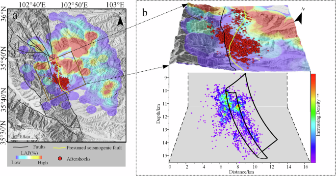
Distribution of aftershocks and location of presumed seismogenic faults.
Despite our efforts to enhance the precision and value of this study, certain unavoidable limitations remain. The spatial resolution of the foundational data is one such constraint; we utilized satellite imagery with a 3 m resolution, which captures most coseismic landslides but may miss smaller-scale events. The 30 m Copernicus DEM, widely used in published research, is among the highest-resolution open-access DEMs currently available. Although higher-resolution DEMs, such as those from UAV surveys, could offer finer detail, limitations in data availability and coverage led to our choice of this dataset. While these factors may introduce some errors, they do not impact the overall trends or influencing factors observed in landslide distribution.
Regarding the seismogenic fault, our study highlights the observed hanging wall effect, further supporting the NE-dipping fault hypothesis. However, more comprehensive structural geology analysis—including the influence of other environmental factors and fault geometry on landslide distribution—was beyond the scope of this study. Future work will aim to address these aspects, particularly focusing on how fault geometry influences landslide distribution.
This study, based on remote sensing imagery, interpreted the landslides triggered by the 2023 Jishishan earthquake and identified a total of 2643 landslide vectors. The characteristics of the coseismic landslides were analyzed, leading to the following main conclusions:
-
1.
Geographical distribution characteristics of landslides: the Jishishan earthquake triggered a large number of coseismic landslides that covered an area of 4.36 km2, primarily concentrated in the central, northeastern, and southeastern parts of the study area. These areas correspond to low mountain hills and river valley plains, with a high degree of overlap with local residential areas. The landslides are predominantly of medium scale, with a few extremely large landslides, such as the liquefaction-induced landslide mudflow in Zhongchuan Township.
-
2.
Influencing factor analysis: through correlation analysis, nine key environmental factors were identified as significant influencers of landslide distribution: elevation, slope, aspect, TPI, slope structure, stratum, distance to rivers, PGA, and NDVI. These factors collectively influence the distribution of landslides. The following ranges were found to have a significant advantage in landslide occurrence: elevation between 1700 and 2300 m, slope angle between 20 and 40°, SE and S aspect, middle slope position, Paleogene and Neogene stratum, transverse and incline slope structures, within 400 m of rivers, NDVI interval of 0.2–0.6, and PGA interval of 0.45–0.6 g.
-
3.
Implications for seismogenic structure: the study discusses various research findings on the seismogenic fault responsible for this earthquake. By analyzing the distribution of landslides in conjunction with the aftershocks sequence, the results support the conclusion that the seismogenic fault is an NW-SW striking, NE-dipping thrust fault. Additionally, the landslide distribution exhibits a clear “hanging wall effect.”
Responses