Long-time error-mitigating simulation of open quantum systems on near term quantum computers

Quantum systems in nature are inherently open—they inevitably interact with an environment, except in extreme cases of perfectly isolated particles. As a prototypical example, we consider condensed-matter systems, where the electrons that exhibit interesting emergent phenomena (such as superconductivity) and their strongly coupled lattice vibrations co-exist with a hard-to-characterize environment that has contributions from, for example, remaining lattice vibrations and spurious external electromagnetic fields. Nevertheless, we observe emergent quantum phenomena in nature, which indicates that the presence of these (typically dissipative) effects does not destroy the emergence of complex quantum physics. This is because the open quantum system has fixed points^1,2 that continue to exhibit the emergent phenomena. Thus, we can theoretically ignore the open-ness, and focus on the emergent phase within an approximate closed-system description.

The situation gets more complicated when driving fields are introduced. Now, the dissipative effects are crucial for determining the fixed point(s), called non-equilibrium steady state(s) (NESS), and thus a full open system needs to be solved. This requires the use of a density matrix formalism, which further exacerbates the “curse of dimensionality” that already plagues pure state simulation. However, this is also a research frontier in many different disciplines: (i) in quantum condensed-matter physics, pump-probe experiments drive a system into nonequilibrium and watch how it evolves³; (ii) in chemistry, driving and dissipation play important roles in photochemistry⁴ and in cavity-enhanced reactions⁵; (iii) in nuclear and high-energy physics, collisions of heavy nuclei induce nonequilibrium dynamics⁶; (iv) in quantum optics, cavity QED studies dressed atoms in a cavity and how they reach a steady state⁷; and many more. In some cases, the system is driven to new (meta)stable non-equilibrium phase that cannot be produced any other way⁸. In this work, we are interested in both steady states that do not change, and limit cycle states, which have periodically repeating “steady states”.

From an applications perspective, many devices rely upon the nonlinear response of the system to external fields—the switchable nonlinear current-voltage curve of a transistor is a classic example. As quantum materials are sought for use in novel device applications, understanding how they respond to fields in the presence of dissipation is critical for engineering these devices. Hence, driven dissipative systems also have an almost ubiquitous appearance through many fields of applied science.

An emergent technique for modeling quantum systems is to use quantum computers. These are naturally open systems by themselves: the qubits interact with an uncontrollable environment. They undergo τ₁ and τ₂ decay, and the fixed point of their evolution is typically the (leftvert 0rightrangle leftlangle 0rightvert) state, i.e., the individual qubit’s ground state. Indeed, much of the progress on today’s quantum hardware is limited by the decoherence of the individual qubits⁹. Efforts are underway to improve this situation, but with an eye towards closed quantum simulation, which is sensitive to the environment, and which does not typically exhibit fixed points in the dynamics. The situation improves when simulating open systems on a quantum computer^{10,11,12,13,14,15}, which is a topic that has garnered some interest recently^{16,17,18,19,20,21,22}.

Here we show that modeling a driven-dissipative system on a quantum computer is intrinsically stable on the hardware, even in the presence of noise and decoherence. The stability happens because the dynamics map all initial states that are not protected in some way onto the fixed point of the evolution, which is a periodic NESS. This naturally includes states that have undergone some perturbation by the noise in the hardware, and in this way, errors incurred in one-time step are corrected by the inherent dynamics in the next step. The fixed point is determined by a combination of the quantum channel corresponding to the evolution of the system under study and the intrinsic quantum channel of the noisy quantum computer. The quantum-computer channel shifts the fixed point slightly, which is borne out in our results, and we show that the clean limit can be obtained via extrapolation of the noisy results. Because of this inherent stability and because these problems are challenging to solve on conventional computers, the driven-dissipative problem is an excellent application for near-term quantum computing.

We illustrate how dissipative quantum simulation can be performed on IBM’s quantum computers by considering two problems derived from the Hubbard model in two distinct limits: 1) a noninteracting system of lattice electrons at finite electric field and temperature; and 2) an interacting single-site two-electron system in a magnetic field that thermalizes—the Hubbard atom. As discussed below, while the free fermionic problem is trivially solvable in a closed system, the presence of dissipation adds significant complications that inhibit a simple solution of the (polynomially-sized) 1-body Hamiltonian.

The key new feature that allows for open quantum system simulation on near-term hardware is the mid-circuit reset gate. There are two ways to use this to simulate dissipation into a reservoir or environment—one way simulates the full system plus reservoir and uses mid-circuit resets to dissipate energy from the qubits that represent the reservoir, while the second way integrates out the reservoir and implements more complicated dynamics involving superoperators. In the first case, one works with a larger Hilbert space corresponding to the system plus reservoir, but the dynamics are unitary time evolution, followed by reset operations on the reservoir qubits which remove energy and create mixed states²². In the second case, one works with the smaller Hilbert space of the system only (and hence can incorporate infinite-sized reservoirs), but the time dynamics is that of a non-unitary quantum channel, which is more complicated to implement. In this work, we follow the second approach.

Approach

Although many quantum algorithms are known for the simulation of closed quantum systems, fewer studies have considered the simulation of open quantum systems despite their rich and interesting behavior²³. Current approaches using inherent qubit decoherence^15,24,25, direct simulation of an environment^26,27,28, implementing Kraus maps/Lindblad operators^{20,29,30,31,32,33}, variational techniques^34,35, and more^36,37. Since Barreiro et al. first demonstrated their open-system quantum simulator³⁸, current early-stage dissipative simulations of quantum systems in the areas of quantum chemistry and physics^{15,17,19,20,21,22,30,36,39} have been completed. Here, we implement a Trotterized driven-dissipative map, which involves the application of Kraus operators at each time step^{20,30,31,32,33}. On a quantum computer where the natural operations are unitary, we implement the non-unitary gates by coupling to an ancilla qubit which is subsequently reset; this produces a non-unitary channel resulting in an eventual (mixed) state.

For our models, we choose two endpoints of the interacting Hubbard model. The first endpoint (noninteracting lattice electrons) is a system of free fermions in the presence of infinitely sized dissipative bath; the second endpoint (interacting electrons on a single site) is the Hubbard atom. Note that, in stark contrast to the closed system case, where free fermionic models are exactly solvable, the addition of dissipation renders the model to be non-trivial. An exact solution for a metal with a constant density of states does exist⁴⁰, but it is not trivial to obtain; it requires using the Keldysh Green’s function formalism to complete it. The choice of an (integrated out) infinite bath is critical to avoid finite-size effect oscillations that arise from directly simulating the reservoir²², which inhibits the stability of the fixed point.

We underscore that all of the steps that need to be implemented are the same for a non-interacting system as for an interacting one. The main differences are that (i) by working in the single particle basis, the Hilbert space is much smaller for the non-interacting system, and (ii) that the computational basis is the appropriate basis for the Kraus operators. Interacting systems are primarily complicated by the nontrivial basis needed for the Kraus operators; when exactly integrating out a reservoir the number of Kraus operators is given by the square of the Hilbert space dimension, and they map energy eigenstates to energy eigenstates, making this “straightforward” approach impossible to carry out on a quantum computer, except for very small systems. Thus, although our demonstration does not cover the full range of systems, the approach can be extended more broadly once an efficient representation for the Kraus operators is found, or other more efficient algorithms are discovered which allow single-time steps to be carried out with high enough fidelity.

The concrete details for how we determine the algorithms here are given in the Supplementary Information. The specific systems we study have the benefit that the computational basis is a natural basis for the Kraus operators, which allows their implementation to be quite efficient. In addition, many of the Kraus operators are not needed to achieve the desired time evolution. This is because we are not simulating a specific reservoir, but instead are simulating a generic one. In the case of the Hubbard atom, because we are going to a thermal state, and this state can be universally prepared by any thermal reservoir, we can greatly reduce the number of Kraus operators needed. In order to be be able to carry out this work, the most efficient implementation of the open system is required in order to have sufficient fidelity for each Trotter step.

Infinite 1D chain of driven-dissipative fermions

First, we examine the free fermion limit of a Hubbard model in the presence of a driving field and dissipative coupling to a bath. Electrons freely move on an infinite one-dimensional lattice via nearest-neighbor hopping (used as our energy unit), with semi-infinite electronic thermal reservoirs (taken in the wide-band limit) attached to each lattice site. A DC electric field of strength E is applied by employing a linearly varying Peierls phase ϕ(t) = Ωt (Ω = eEa, with e the electric charge and a the lattice spacing (we set ℏ and c to one) in the lattice hopping parameter γ_h. The system Hamiltonian reads:

where ({d}_{i}^{dagger }/{d}_{i}) are the creation/annihilation operator of the electrons. Each lattice site is coupled to a reservoir by hopping term to one end of a semi-infinite reservoir with Hamiltonian ({hat{{mathcal{H}}}}_{b}={sum }_{ialpha }{omega }_{alpha }{c}_{ialpha }^{dagger }{c}_{ialpha }), where ({c}_{i}^{dagger }/{c}_{i}) are the creation/annihilation operators for the bath, using a coupling term (hat{{mathcal{V}}}=-g{sum }_{ialpha }({d}_{i}^{dagger }{c}_{ialpha }+{c}_{ialpha }^{dagger }{d}_{i}).) Here g is the bare hybridization amplitude, and α is an index that runs over all the internal degrees of freedom of the bath, which are taken to be infinite. As we show in the supplement, after integrating out the bath, the properties of this coupling can be summarized in a parameter Γ given by the square of the lattice-reservoir hopping multiplied by the density of states of each reservoir.

The infinite system is diagonalized by Fourier transforming to momentum space. In this fashion, the dynamics of the infinite lattice is addressed by solving many independent single-qubit systems, each of which depends on the specific value of the crystalline momentum k; in the steady state, we construct the results for all momenta from the results for any single momentum by invoking gauge invariance. The key point is that a constant DC electric field shifts the momentum linearly in time (when we employ the Peierls substitution). This means that the results from different momentum values can be found by simply shifting the time axis of the results for one momentum (further details are presented in the Supplementary Information). Hence, the properties of the infinite lattice can be determined by the results for the time trace of just one momentum. The time and momentum-dependent Kraus operators (for the time step of duration Δt) are given by:

where ({d}_{k}^{dagger }) is the creation operator of a lattice electron with momentum k, ϵ_k(t) is the time-dependent dispersion relation, Γ is the strength of the coupling to the reservoir (here set to 0.1), and n_F(x) = 1/(1 + e^βx) is the Fermi-Dirac distribution at the temperature of the reservoirs (here set to (beta =frac{1}{{k}_{B}T}=5)).

From the Kraus map given in Eq. (1) the quantum circuit can be constructed¹⁰ and appears in Fig. 1d. Note that this particular circuit produces the correct time evolution for the diagonal elements of the density matrix; if desired, off-diagonal elements can be obtained by rotating the basis such that these are diagonal. The (leftvert 0rightrangle) gate in the circuit is a reset operation which ideally sets the qubit to the (leftvert 0rightrangle) state. However, this operation is not perfect on current hardware and the reset fidelity can be improved by applying it to a qubit multiple times in succession (at the cost of additional amplitude damping on the remaining qubits because the reset operation takes by far the longest time to run compared to the rest of the circuit). We run our circuit using one to four reset gates per Trotter step. This data is used to build an effective model of the error combining these two effects, which we use to extrapolate away some of the errors. Details are given in the Supplementary Information.

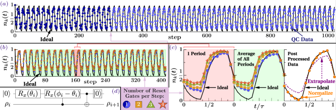
a 1000 steps of time evolution on ibmq_mumbai using one reset gate per Trotter step. Reported data has been corrected for measurement errors. Statistical errors are at about the 1.5% level, smaller than the size of the plotting symbol (so error bars are suppressed). Different shades of blue represent different sets of qubits while the solid black line is the ideal result of running the circuit. b 400 steps of time evolution on ibmq_boeblingen using one to four reset gates in succession per Trotter step. Reported data has been corrected for measurement errors. c Left panel shows a zoom in on one period of the data shown in (b). Middle panel shows one period of data obtained by averaging together all periods of steady-state data (step > 30). Right panel shows post-processed averaged data as described in the technical details section. d Quantum circuit for one Trotter step of time evolution. Here, ({theta }_{i}=2{sin }^{-1}sqrt{frac{2Gamma Delta t}{{e}^{beta {varepsilon }_{i}}+1}}) and ({phi }_{i}=2{sin }^{-1}sqrt{frac{2Gamma Delta t}{{e}^{-beta {varepsilon }_{i}}+1}}) where ({varepsilon }_{i}=-2cos (k+Omega iDelta t)) is the dispersion relation at step i (at time t = iΔt), and we use Γ = 0.1.

Full size image

Figure 1a plots the results of running the circuit shown in 1d with a single reset gate per Trotter step. The first 300 steps were run on one set of qubits and the remaining 700 on a second set. These runs are robust both with respect to the choice of qubits and with respect to the total time of the run. The circuit for the 1000^th step required 2000 CNOT gates and yet the data show no sign of a decaying signal. Note that the transients have died off after about 30 Trotter steps. In panel (b), the raw data with one to four resets is shown for up to 400 Trotter steps. After processing the data via extrapolating to the zero-reset-time limit and then correcting the result by shifting and stretching as described in the SI, one can see that the post-processed data (c) agrees with the exact results to high precision. This simulation clearly shows the stability of driven-dissipative circuits on near-term quantum computers, producing accurate time evolution far longer than is currently possible with the quantum simulation of coherent dynamics of electrons⁹.

Figure 2 shows the steady-state DC current response (averaged over one oscillation) of the system to an applied electric field, and compared against the ideal circuit and theoretical results from Lindblad techniques, as described in ref. ¹⁰. We can see an interesting result has developed. The Bloch oscillations that are characteristic of free electrons in an electric field in the presence of a heat bath in our model give rise to a net DC current. As a function of external field, the current first increases as expected because more energy is put into the system, but soon reaches a maximum and then decays. The reason for this is illustrated by the inset of Fig. 2, which shows that as the electric field is increased, there are more oscillations, and integrated, these cancel out. One can see that the maximum current is characterized by minimal transient oscillations.

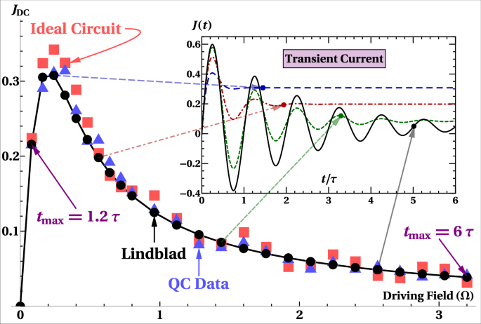
Comparison of the DC response at a given field strength as computed (see technical details section) using: (i) the Lindblad master equation (black circles), (ii) the ideal circuit (red squares), and (iii) the measured data from ibmq_boeblingen (blue triangles). All circuits for the current were run for 50 Trotter steps each due to total quantum computer time available, leading to a trade-off between Trotter error and convergence error. Δt was chosen empirically such that Δt/τ is linear in Ω. Convergence to the steady-state current is shown in the inset with the solid dots representing ({t}_{max }) for that run.

Full size image

That the transient region extends to longer times as the electric field is increased has practical ramifications as well, requiring the simulation to run further in time. Hence, the calculation requires a trade-off between Trotter error (large time step size) and convergence error (steady state not yet reached). To minimize the total error, we choose Δt empirically with Δt/τ ≈ 0.022 + 0.031Ω (here, τ = 2π/Ω). At large driving fields it is clear that we have not yet reached the steady state and oscillations in the DC current data are observed even in the ideal case. At small driving field (Delta t={mathcal{O}}(1/Omega )) and we incur large Trotter errors. Despite these limitations, the quantum computer results match both the ideal circuit and the theoretical results fairly accurately across the entire range of simulated field strengths.

Interacting orbital with magnetic field and baths

The second problem we simulate is the atomic limit of the dissipative Hubbard model in an external magnetic field B, where the bath may be either hotter or colder than the system. This system with maximum two electrons is a strongly correlated electron problem, which can be simulated with four qubits. The energy cost of double occupancy is given by U and the magnetic field shifts the energy levels of the single-spin states up or down with an energy splitting given by B, measured in units of the Bohr magneton. The Hamiltonian is

where U is the on-site interaction strength, μ is the chemical potential, B is the magnetic field in units of energy, and n_α is the occupation number operator for state (leftvert alpha rightrangle). B is chosen to have a sign such that energy is lowered by the occupation of a single up electron.

We build our dissipative circuit by using Kraus operators that induce transitions between computational basis states, which are the energy eigenstates. These transitions are implemented by mapping the system state to an ancilla register and rotating the system qubits controlled on the ancilla^10,38 (shown in Fig. 3a); the approach uses just the transitions that correspond to a cycle through the states (depicted in Fig. 3b) Details are given in the Supplementary Information. This circuit is iterated N_T = 19 times to simulate N_T Trotter steps of time evolution.

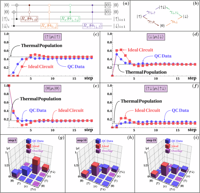
a Circuit for a single Trotter step of time evolution. The rotation angles Θ are given in terms of transition probabilities γ, which are derived from the detailed balance condition as depicted in (b) and described in SI. ({Theta }_{i,j}=2{sin }^{-1}(sqrt{{gamma }_{i,j}})) and ({gamma }_{i,j}propto {e}^{beta {varepsilon }_{i}}), where ε_i is the energy of state (leftvert irightrangle). c–f Results showing the populations of each of the four possible occupation states versus Trotter step for the ideal case (red squares), measurement-error mitigated data from ibmq_mumbai (blue circles), and the theoretical thermal population (dashed black line). g–i Full tomography of the density matrix at selected time steps.

Full size image

Figure 3 shows the transient evolution of the Hubbard atom from the vacuum state (with no electrons) to a thermal state with filling n ≈ 0.83 at a temperature T = U/2 in an external magnetic field B = U/4 using one reset per Trotter step. We note the effect of finite temperature on the results. Indeed the state parallel to the magnetic field (c) has the highest population at steady state, but it remains below 1/2. The next highest population is the state with one down electron (d), which although paying a cost of being opposite the magnetic field, still is not causing a Coulomb interaction U. Note the relatively large fluctuation to large population for the one down electron as the filling is ramping up from vacuum state, partly a result of noise, but mainly because (see the directionality of the arrows in Fig. 3b) this state is filled first from the vacuum. The state with no electrons (e) is, of course, the initial condition, so it shows occupancy 1 at step 0, but soon drops to low occupancy, but not so low as the state with two electrons (f), which suffers the energy cost U.

These data are only post-processed for measurement-error corrections. The transient data lie close to the ideal circuit but show deviations due to intrinsic errors in the hardware. Nevertheless, the steady state is reproduced accurately for the four different populations of the thermal state (c–f) and for the thermal final density matrix (g-i). This further exemplifies the robustness of these types of algorithms to noise and how errors in early time steps are largely corrected in subsequent steps.

In this work, we have demonstrated that the capabilities of near-term quantum hardware for simulating open quantum systems are greater than one might expect based on the state-of-the-art results in simulating closed systems. By making use of the newly developed reset gates and mid-circuit measurements, we have achieved dynamical simulations, with 1000 Trotter steps using circuits of up to 2000 CNOT gates with minimal signal decay. We interpret this success by viewing the dissipative dynamics as a dynamical map with a fixed point; the hardware noise is not sufficient to overcome the tendency of the map to drive the systems towards their respective fixed points. It may perturb the fixed point but does not significantly modify its character, which is what makes the process robust.

For the models discussed here, we observe that the dynamical map of the evolution has a unique fixed point and that the fixed point is only mildly affected by the hardware noise and the Trotter time-step infidelity. This is evidenced by the relatively good agreement between the ideal circuit and the QC data shown in Figs. 1 and 3. In general, however, it may be that in other scenarios the fixed point is sufficiently sensitive to the particular effects of the noise that the resulting evolution retains very little of the ideal circuit. Similarly, we expect that as the noise gets worse, for example when scaling to larger systems, that the modification of the dynamical map becomes more severe. We reserve these questions for future investigation. However, we do note a simple empirical result; if a single Trotter step has sufficiently high fidelity—i.e., the map of the open system combined with the intrinsic decoherence of the quantum computer and the infidelity of the Trotter step yields a fixed point that is close enough to the fixed point of the original open system—then the simulation is successful and can be accurately continued to long times. This result is similar in nature to the well-known result for error correction that the fidelity of the individual qubits must be sufficiently high in order for it to be possible to carry out error correction. The analog here is the sufficiently high fidelity of a single Trotter step.

These conclusions bring up an important question—under what circumstances will the perturbation of the fixed point be small and controllable so the quantum simulation will be successful? We are not able to answer this question here, and we believe it is an important question for the community to address given the results we have found, which indicate rather broad robustness. In order for these types of problems to be solved on quantum computers knowing which systems will be successful and which ones will fail is obviously an important area for future work.

The community is searching for nontrivial problems that can be solved on quantum computers that show an advantage over classical computers. While our work has not yet achieved this goal, it does show that this class of problems is a potential path towards achieving this goal. Aside from our demonstration here, another reason is that the non-equilibrium many-body problem does not have efficient algorithms to solve it on classical computers. The algorithms that do exist usually are restricted to either very small-size systems or to short times. Here, we show that on a quantum computer, there may not be a short-time restriction, and this is a very important result for using them to simulate nontrivial systems.

All data were taken using superconducting quantum computers made available by IBM, either ibmq_mumbai (Figs. 1a and 3) or ibmq_boeblingen (Figs. 1b, c and 2). ibmq_boeblingen is a 20-qubit quantum device and ibmq_mumbai is 27-qubit device. These two devices were chosen because they were among the first with reset gates available. The reported error rates were used to select sets (~5–10) of candidate qubits on which a limited number of Trotter steps were run. Results from these were then used to select the final qubits on which the full job(s) would be run. Raw shot counts were processed using Qiskit Ignis’⁴¹ built-in measurement error mitigation protocol. This prepares and immediately measures each computational basis state giving a confusion matrix, which is inverted and applied to the raw shot counts to yield the mitigated shot counts. For each data point shown in the figures, we used 1000 shots.

This work pushed current near-term quantum computers to their limits. This created some unique issues when trying to run these extremely deep circuits. We encountered buffer overflow errors after running a large number of our larger circuits indicating we had overflowed the device’s capacity to record more measurement data. This is why we limited our DC current data to 50 Trotter steps per unique set of parameter values. We avoided this limit when taking data for Fig. 1b by breaking our jobs into smaller chunks, but this meant long queue times, which would have been prohibitive to get the data in Fig. 2. The data in Fig. 1a were obtained through exclusive access to ibmq_mumbai, which allowed us to break our circuits into individual jobs without worrying about queue times. Nevertheless, we still overflowed the buffer around step 300, forcing us to change to a new pair of qubits with a fresh buffer. Finally, we began to exceed the limits of the system generating the driving microwave pulses at around 1000 Trotter steps, which is why this is the upper limit for Fig. 1a.

For the full tomography results in Fig. 3, we made use of the “state_tomography_circuits” function and “StateTomographyFitter” class built into Qiskit Ignis. The “state_tomography_circuits” creates a list of 3ⁿ circuits which carries out the desired quantum circuit and then measure in the X, Y, and Z bases. These results are then fed into the “StateTomographyFitter.fit” function in order to reconstruct the full quantum state.