Loss formulations for assumption-free neural inference of SDE coefficient functions

Introduction
Stochastic differential equations
Stochastic differential equations (SDEs) are a class of equations widely used to describe continuous-time dynamical systems, including many complex biological and natural processes. The most commonly studied form, also known as an Itô equation, can be represented as
where a is the drift coefficient governing deterministic dynamics, b is a diffusion coefficient representing the variance of noise impacting the evolution of the system, and Bt represents Brownian Motion (see1,2 for a rigorous account on stochastic integration). Intuitively, they can be understood as a middle way between two contrasting levels of modelling granularity: Microscopic interacting particle systems can accurately depict individual variability but are often computationally intractable. By contrast, macroscopic ODE modelling, is computationally and theoretically well-understood, but may provide insufficient information about intra-population variance. From this view, SDEs represent a mesoscopic scaling regime where the influence of many small random interactions is summarised into the diffusion term, but not eliminated fully. This makes them an attractive choice for biological modelling3,4,5 as well as other fields such as engineering6, epidemiology7 or finance8.
While the study of parametric SDE inference is deeply developed, the problem of recovering coefficient functions from data without any assumptions on the analytical structure has received far less attention. Research in this direction is being done using neural networks, whose universal approximation property and ease of optimisation have in the recent past driven a highly active area of research on the intersection of deep learning and dynamical systems theory9,10,11. It broadly falls into two philosophical categories:
One view, often referred to as the neural differential equation12,13 approach, sees time series data as realisations of a generative neural network, which thus represents not just analytical dynamics but instead a sort of “solution operator”. Here, deep learning can serve as a tool towards performing inference14 on, or sampling from a differential equation system. Notably, Ryder et al.15 considered trajectories as samples from a variational RNN; more recently, Kidger et al.16 proposed the SDE-GAN method for re-interpreting them as samples from a generative adversarial model. In all these cases, the goal is to obtain a system that can produce new sample paths sampled from the SDE underlying the training data – in other words, to sample from the solution distribution. For a comprehensive treatise on these and related methods, we refer the reader to the highly influential work by Kidger13.
The other view, from which we undertake the proposed study, instead emphasises the role of a neural network model to fill in unknown elements of some predefined dynamical system. Pioneered by Rackauckas et al.17, and termed universal differential equations, its key aim is to enable discoveries about underlying models, for which deep learning is an instrument; in this interpretation, neural networks represent functions, not full systems18,19. For ordinary differential equations, and under certain assumptions on the involved kinetics, the use of deep learning has been proposed to facilitate parameter estimation19,20, but also for dynamics discovery21 via symbolic regression.
For SDEs, however, there is little established work beyond that of Rackauckas et al.17, who represented coefficient functions as a neural network, and subsequently optimised it by penalising disagreement between observed data and simulations from the current coefficient model candidate. It is this approach upon which we aim to improve (see also Fig. 1 for an overview), as we
-
present the novel idea of utilising pseudo-likelihoods – already a well-regarded tool in parametric inference22 – as an alternative objective function,
-
suggest more robust loss formulations for the existing, simulation-based, methods, and
-
show that the two approaches can successfully be hybridised to greatly improve on the performance of either one.

Observed data serves as the basis for inference on the underlying coefficients.
As working with SDEs is a universally challenging endeavour, we lay no claim to having produced a universally optimal approach to SDE inference. However, we hope to demonstrate that the ideas we propose already provide a significant improvement on existing methods – as demonstrated by extensive benchmarking – and have great potential for the further development of robust inference algorithms.
Results
Combining simulation-based and pseudo-likelihood objectives yields a flexible hybrid formulation
In this study, we propose the Hybrid Lie-Trotter loss for a neural network representing the coefficient functions, derived in detail in section 4, whose components are
-
1.
the Wasserstein distance between observed and re-generated samples’ empirical distributions,
-
2.
a negative log-pseudo-likelihood of the observed sample paths given the model, and
-
3.
the discrepancy between observed a re-generated samples’ empirical auto-correlation.
In the following, we present the result of all evaluation metrics to compare the proposed Hybrid Lie-Trotter scheme and the respective state-of-the-art, – Moment matching as proposed by Rackauckas et al.17 for all three metrics taking the ground truth into account, and SDE-GAN16 for the last, comparing solution distributions only. We examine a number of datasets, described in detail in section 4. In all tables, we abbreviate Ornstein-Uhlenbeck as OU, Cox-Ingersoll-Ross as CIR, the Unstable Sine problem as SIN1, and the Multi-Modal Sine problem as SIN2. The biological GFP transfection dataset is abbreviated GFP. In all cases, an asterisk denotes the state-of-the-art method, and the best scores are shown in boldface.
Hybrid loss functions outperform other approaches for coefficient reconstruction
To assess the studied models’ capacity for accurately inferring drift and diffusion coefficients of paths from data, we evaluated the expected L2 error of model predictions compared to the ground truth. We found that the proposed hybrid loss yielded results that are significantly better than the state-of-the-art moment matching method (see Table 1).
Between the different combinations of loss terms that we studied, we found hybrid schemes to outperform lone pseudo-likelihood-based and lone simulation-based losses in all cases. For a detailed summary of all scores for drift and diffusion coefficient reconstruction, see supplemental Tables S1 and S2 respectively.
Evaluating the results of the diffusion coefficient estimation was more difficult as most methods very accurately approximated the diffusion coefficient functions. Here, too, however, the proposed hybrid scheme – while not technically the best for any problem – always had a performance nearly indistinguishable from the best model.
The proposed method provides higher accuracy for newly generated samples
For the problem of generating samples from the solution distribution, we performed the experiment of generating sample paths with either true or estimated dynamics, and the same initial condition and driving Brownian Motion sample paths. Here, too, we reported the L2 error and found the hybrid schemes to fare much better than individual losses, and in particular than moment matching (see Table 2; as well as, for example, Figs. 2 and 3 for the visualisations of the results on the Ornstein-Uhlenbeck and GFP data, respectively).
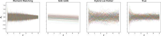
Results after optimisation are shown for the state-of-the-art as well as the proposed method, and compared to the true test set.
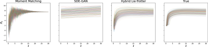
Again, results after optimisation are shown for the state-of-the-art as well as the proposed method, and compared to the true test set.
As before, in the comparison of all loss combinations, no one method proved best for all problems (see supplemental Table S3 for a full breakdown of achieved scores), but hybrid approaches always outperformed moment matching. In our final evaluation, we evaluated the signature transform metric to also allow comparisons to the SDE-GAN method and for problems without a ground truth. With respect to this metric, too, we found that the proposed scheme outperformed the state-of-the-art (for the detailled results, see supplemental Table S4).
From the perspective of purely sampling from the solution distribution, measured in quality by maximum mean discrepancy from testing samples after depth-5 signature feature transform, there was a very wide spread of scores across problems and methods, but the proposed loss functions combining pseudo-likelihoods, the Wasserstein, and the auto-correlation losses outperformed the state-of-the-art SDE-GAN method in all cases (see Table 3).
Simulation time is a decisive contribution to computational cost
Evaluating the runtimes of the different methods, we could – unsurprisingly – observe that methods that generate synthetic samples as part of the loss function evaluation take the largest computational effort to train (for a full runtime comparison, see Table 4). Compared to the Euler-Maruyama pseudo-likelihood, the calculation of second derivatives that is necessary for the Lie-Trotter scheme creates additional overhead, but its magnitude is insignificant compared to the simulation overhead (of course this depends strongly on the number of trajectories generated in each optimiser step, but should be true for any reasonable number of synthetic paths).
A direct comparison of runtime to the SDE-GAN approach was not possible, as the methods were executed on different machines. However, we can confidently say that the SDE-GAN training is more computationally intensive by orders of magnitude, as 100 epochs of training required approximately 68 hours on a GPU node in a computing cluster, while all other models trained in less than two hours on a consumer-grade CPU.
Discussion
In this study, we investigated the problem of inferring SDE coefficient functions from data given no assumptions on analytical structure. We introduced the existing methods and the core idea of representing the structurally unknown dynamics of a differential equation system by a deep neural network, and proposed a novel objective function formulation, which combines strategies from simulation-based inference and classical approximation methods, penalising both discrepancies between observed and re-simulated data, and the negative pseudo-likelihood induced by the Lie-Trotter scheme. The advantages of its combined formulation can be gleamed by considering the issues faced by the two respective loss function concepts: The simulation losses that penalise discrepancies of marginal distributions efficiently control population summary statistics, but the behaviour of individual paths can become extremely erratic; pseudo-likelihood optimisation, by contrast, controls the behaviour of individual sample increments, but can infer no information in areas of phase space with little or no data, leading to the danger of diverging sample paths. Thus, the two approaches, when hybridised, efficiently address each other’s shortcomings (see supplemental Fig. S1 for an illustration of the regularisation provided by increasing the weight of the Wasserstein term). As a result, the evaluation on both synthetic and real-life data showed that this combined loss formulation consistently performs better than the state of the art, and qualitatively captured the dynamics of the different datasets well.
The next step towards using the presented system for obtaining biological insights would be to identify analytical structure behind the data, leading to the field of symbolic regression. Initial experimentation with a method recently proposed by Cranmer et al.23 has proven promising on the simple Ornstein-Uhlenbeck example; but has so far not resulted in reliable mechanics identification for the more complex problems, suggesting a need for further investigation. To make the results of dynamics discovery more interpretable and reliable, uncertainty quantification on the estimated coefficient functions would be of great value, e.g. using Bayesian Neural Networks24. We have not been able to use them to produce consistently robust fits, but believe that technological advances may overcome this limitation. For the SDE-GAN method, we observed a broad failure to train with the procedure and hyperparameters in16, despite copying the original setup, observing an imbalance in training as the generator loss continuously increased – we hypothesise that this could be due to vanishing gradients if the generator initialisation is too far away from the true distribution and it cannot produce credible sample paths; however we were not able to pinpoint the exact reason, or obtain a better hyper-parameter configuration.
All experiments we considered, including the real-life biological data, were in a dense-data regime. More research is needed on possible adaptations to data sparsity, which occurs often in applications. Given larger time steps, we would expect them to impact the less stable Euler-Maruyama pseudo-likelihood more strongly than the other loss components. To build a system more robust towards data sparsity, however, there are a number of possibilities. The most promising, in our opinion, would be to co-opt strategies often utilised in classical parametric inference, such as bridge re-sampling approaches22,25 which repeatedly iterate between re-sampling paths based on the current model and updating the model based on the imputed data. While in our study we utilised a simple forward scheme for simulating sample paths within the loss function evaluation – in order for it to remain compatible with automatic differentiation and thus the neural network training –, future work would certainly benefit from the use of automatically differentiable implementations of higher-order solvers, such as those in the growing Diffrax library13. Given sufficient data density, on the other hand, another promising avenue would be de-coupling the tasks of estimating the drift and diffusion, thus utilising a timescale separation approach, as has been suggested by Ditlevsen in the context of climate modelling26.
The overall evaluation of our results showed, most of all, that SDE inference without any structural assumptions remains a formidable challenge. At the same time, our contributions provide a significant increase in estimation quality compared to the state-of-the-art, and we see them as a stepping stone towards a more comprehensive framework for stochastic dynamics discovery from data.
Methods
Assume that we observe a set of trajectories (X={({X}^{(i)})}_{1le ile N}), of which each is sampled at a set of discrete time points ({({t}_{k})}_{k}). They are assumed to be realisations of a strong solution to some SDE in the form of equation (1), with no prior knowledge about the analytical structure of the functions a, b. The objective is now to train a neural network to represent these unknown functions, which map from (t, x)-phase space to scalar drift or diffusion, respectively. Given a good fit, this can be used to investigate the dynamics, but also to sample anew from the solution distribution. This naturally depends on an advantageous loss function to quantify disagreement in terms of empirical moments between network predictions and actually observed data.
The most natural choice, would be to directly apply maximum-likelihood estimation: If we observe a transition from state x at time t to ({x}^{{prime} }) at time ({t}^{{prime} }), we would like to access the solution’s transition kernelπ, yielding our desired objective, given candidate functions (hat{a}), (hat{b}),
where Y solves
Unfortunately, except for very few cases, this likelihood is intractable. Even when the dynamics are structurally known, few SDEs admit an analytical solution, and fewer still an explicit transition density. In our “assumption-free” case, there is no way at all to grasp at this object – numerically or otherwise.
The avenues that remain open are similar to those in other domains and contexts where direct likelihood evaluation is impossible:
-
Either circumventing it completely by using a simulator for the studied dynamical system (Methods of this kind are frequently referred to as “likelihood-free” and appear in numerous applications27, especially Bayesian learning28), or
-
making do with some approximation of the likelihood, if a reasonable choice exists.
Simulation-based learning
Employing a simulator, which in our case is any SDE solver, to address the inaccessible likelihood can be done in a straightforward fashion. By generating a number of SDE trajectories from the current network state, and comparing summary statistics with those obtained from the observed data, we can quantify the dissimilarity between the real and estimated dynamics.
To put this into formulae, let (Xin {{mathbb{R}}}^{Ntimes T}) denote the data consisting of N independent trajectories at T timepoints. Moreover, let Ξ, here and in the following, denote the SDE solution operator with some abuse of notation: Given coefficient functions a, b, we write Ξm(a, b) to denote m independent paths sampled from the solution of the SDE in equation (1).
Moment matching
To compare simulated to real samples, Rackauckas et al.17 have proposed using moment matching. They suggest constructing a loss by considering timepoint-wise population means and variances
where (hat{{mathbb{E}}}) and (hat{{mathbb{V}}}) denote the timepoint-wise empirical mean and variance, respectively. Among the approaches directly recovering the coefficient functions, this is the state-of-the-art.
Wasserstein penalty
While the mean and variance provide a good first grasp of the properties of a probability distribution, it is well-known that distributions can have a “moment distance” of zero yet vary wildly even if they coincide in infinitely many moments29. This motivates us to propose the Wasserstein metric, which is widely considered as more robust in other applications30. Given some measures μ, ν, it is defined via the minimisation problem
where Π(μ, ν) is the set of couplings, i.e. joint measures whose marginals are μ and ν, respectively. In particular for the case p = 1, ({{mathcal{W}}}_{1}(mu ,nu )) can be intuitively interpreted as the amount of “work” necessary to reach ν from μ (or vice versa) by shifting probability mass, and thus provides a much more holistic quantification of the distance between measures.
Similar to the moment loss formulation above, we can use it to penalise differences in finite-dimensional distributions between observed and generated samples. We opt to penalise both the average and maximum loss, so that irregularities at specific timepoints are not overshadowed by overall agreement. Thus, we set
where ({hat{{mathcal{W}}}}_{1}) is the timepoint-wise Wasserstein metric.
Auto-correlation matching
The previous summary statistics considered differences between the finite-dimensional distributions of observed and simulated samples, i.e. a population’s collective properties at discrete time points. An alternative approach is to consider trajectories’ empirical relation. Intuitively, while marginal sample variance will describe the typical variation experienced by a population, the auto-correlation will instead measure the typical variation experienced by an individual. This promises to alleviate an often-seen problem with underestimating the diffusion coefficient’s magnitude when the drift is “too flexible” and can itself explain a majority of the (in truth random) variation.
We define, for some lag k and truncation parameter K, the lag-k–autocorrelation
to set
Pseudo-likelihoods
While solutions to SDEs are infinite-dimensional stochastic processes, in a computational setting one uses solution algorithms to approximate them at discrete timepoints. In this context, it is reasonable to hope that the transition kernel of a solution may also be approximated by the transition kernel of an approximation scheme (if that one is in fact tractable). This idea gives rise to the concept of pseudo-likelihoods (which we will denote by Λ to avoid confusion with losses).
These expressions approximate the likelihood of observing a particular transition assuming coefficient functions a, b
and are then converted to losses by aggregating them over all transitions observed in the data. For any method M presented below, we will set
Euler-Maruyama
The Euler-Maruyama scheme31 is the oldest and most well-known solution scheme for SDEs. It is a direct extension of the forward Euler scheme for ordinary differential equations, and relies on the approximation
It immediately follows that
If we now denote by ΛEM the explicit pseudo-likelihood of the scheme above, it holds that
Lie-Trotter splitting
The Lie-Trotter splitting scheme is an approximation algorithm for SDEs that relies on the well-known Lie product formula and was first proposed by Bensoussan et al.32. Its idea is to introduce auxiliary functions to split up the process evolution into a purely deterministic ODE update and the stochastic rest.
Pilipovic et al.33 show that it, too, possesses an explicit pseudo-likelihood and provides formulae. In our case, where the drift and diffusion are fundamentally nonlinear, they are reduced to
It thus becomes evident that for our case, this more sophisticated scheme simply introduces a second-order term into the drift approximation. For a more detailled derivation, we refer the reader to ref. 33.
Combination approaches
From a conceptual point of view, the two presented classes of approaches are complementary in the sense that they address each other’s most obvious weaknesses: Pseudo-likelihood-based methods do not provide any information about the regions of phase space with no data, while simulation-based methods may not sufficiently control the local behaviour of individual trajectories as long as the overall summary statistics remain matching.
It is therefore only natural to introduce loss functions that simply add up both simulation- and pseudo-likelihood-based penalties. Specifically, we propose a combination loss to which we will in the following refer to as Hybrid Lie-Trotter:
for a weighting constant η. Despite its simplicity, we will demonstrate that ceteris paribus, it consistently outperforms both the current state-of-the-art of only matching moments and alternative formulations. (For a brief visual summary of the notions behind the individual loss terms, see Fig. 4).
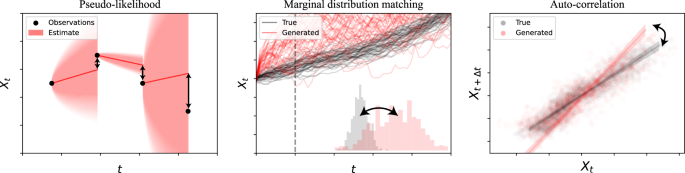
Pseudo-likelihood penalties aim to control the behaviour of individual increments, while simulation-based losses match population statistics.
Experimental evaluation
To rigorously evaluate the different methods’ performances, we study five datasets (directly randomly split into 80% training and 20% test data), of which four are synthetic and showcase different kinds of dynamics SDEs can exhibit. The fifth consists of real experimental data collected and analysed by Fröhlich et al.34 in the study of mRNA translation dynamics, which presents an application example of innate stochasticity in biological systems.
Ornstein-Uhlenbeck process
The Ornstein-Uhlenbeck process35 is one of the most emblematic examples for an SDE and can be written as
with λ > 0, σ > 0. Note that the drift term induces exponential decay, so that the resulting process will not diverge, and is generally speaking relatively benign, having a single point of attraction at Xt = 0, towards which the drift will push it exponentially (see Fig. 5).
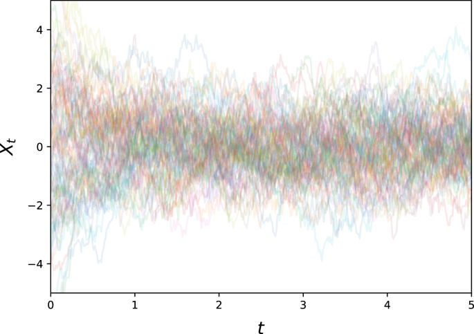
This represents an archetypical noise process with a stable attractor at 0.
We used λ = 2, σ = 2 as example parameters, and generated 5000 paths with initial values samples from ({mathcal{N}}(0,3)). These paths were sampled at 400 equidistant time points for t ∈ [0, 5].
Cox-Ingersoll-Ross process
A step up in complexity is the Cox-Ingersoll-Ross process first introduced by Cox, Ingersoll and Ross36 for the study of interest rates. It is given by
for some α, μ, σ > 0, and thus notably has a non-constant diffusion term. Its drift has a stationary point at Xt = μ towards which it will exponentially gravitate, and is by construction non-negative (see Fig. 6).
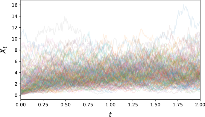
This process is a classical model of volatility, with asymmetric fluctuation around its stable point.
For our simulation of the Cox-Ingersoll-Ross equation, we set α = 2, μ = 4, and σ = 2. We generated 5000 paths, with initial distribution ({rm{Exp}}(1/2)), sampled at 400 equidistant time points for t ∈ [0, 2].
Unstable sine
To provide a higher variety of difficult problem settings, we also study several synthetic datasets with a more challenging coefficient structure. The first is given by
with α, β, γ, σ > 0. It combines two competing effects – Xt = 0 is stable with respect to the γ-exponential decay, but unstable with respect to the sine term. It also features a non-constant diffusion term (see Fig. 7).
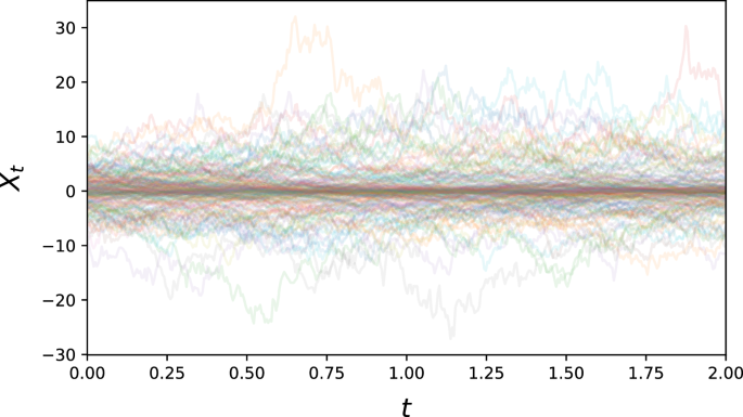
This dataset features increased volatility further away from the (unstable) equilibrium.
For the simulation of the Unstable sine problem, we used the parameter values α = 15, β = (2π)−1, γ = 2, σ = 1.
Multi-modal sine
For a variation on the previous problem, we consider
for some α, β, γ, σ > 0. This equation now has constant diffusion, but time-dependent wells of attraction in phase space, as long as α/γ > 1. Sample paths will typically stay inside an energy well, but occasionally transition given fortuitous realisations of the driving stochastic process (see Fig. 8).
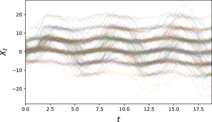
This problem gives an example of multiple time-dependent equilibria.
To simulate the multi-modal sine problem, we set α = 15, β = 1/(2π), γ = 2, σ = 1. 5000 paths with initial condition ({mathcal{N}}(0,{3}^{2})) were sampled at 400 equidistant time points for t ∈ [0, 2].
Biological example: GFP translation
We also perform an evaluation using a published biological dataset34, which contains single-cell-resolution time-lapse data on the translation of transfected Green Fluorescent Protein (GFP) mRNA. Here, all trajectories broadly exhibit the same qualitative behaviour – an initial steep increase in fluorescence, followed by a plateau –, but a high degree of variability can be observed both on the inter-individual (e.g. in terms of maximum fluorescence) and intra-individual (exhibited by noisy behaviour over time) levels. This suggests that the translation mechanism of single cells is still on a sufficiently small scale that stochastic variation arising from its reaction kinetics can be observed directly (see Fig. 9).
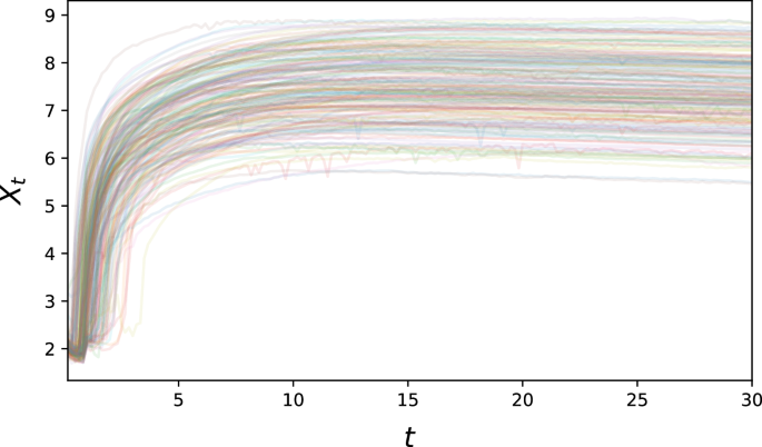
The observed fluorescence intensity is shown in logarithmic scale.
Metrics
To investigate the impact of individual components on the resulting estimates, we examined models trained with each individual loss (the simulation-based Moment and Wasserstein losses; as well as the Euler-Maruyama and Lie-Trotter pseudo-likelihoods), as well as combination losses made up from pairs of the two classes – in all cases either with or without auto-correlation matching.
To compare the quality of newly generated samples from the trained models, we also ran the SDE-GAN method, which is the state-of-the-art for generative SDE modelling, with the same set of hyperparameters as used for the non-synthetic evaluation datasets in13.
The question of how to assess model performance is in itself not trivial, as there are (similarly to the choice of loss function class) two philosophically different approaches: A trained network’s predictions can either be contrasted against true coefficient functions in the examples where this is possible, or evaluated based on their ability to re-generate sufficiently similar trajectories when used for SDE sampling.
Direct coefficient reconstruction
We aim to accurately infer unknown SDE coefficient functions from data. As such, the most natural evaluation approach is to compare the learned coefficient functions directly to the real ones. For this purpose, we sample points in phase space randomly from test data, and report the average L2 discrepancy between the true and estimated drift and diffusion values.
Re-sampling quality
In order to evaluate models’ capacity for re-generating samples from the correct distribution, we simulate new sample paths both from the true and estimated dynamics, using the same initial conditions and driving Brownian Motion sample paths, before comparing the L2 discrepancy.
Additionally, in order to be able to provide a comparison to the SDE-GAN method in terms of re-sampling performance, we followed the evaluation in ref. 16, utilising the maximal mean discrepancy (MMD) metric on the depth-5 signature transform as described by Kiraly et al.37,38.
Implementation
All presented loss functions were implemented in TensorFlow39, using the Euler-Maruyama scheme as the simulator inside the loss evaluation. To avoid numerical issues, all data were scaled by maximal absolute value to [−1, 1] for training; the resulting model predictions were scaled back accordingly. We set the pseudo-likelihood scaling constant η = 10 for all problems, intended mainly to ensure that all loss terms have roughly the same magnitude. For comparing sample auto-correlation, we chose a lag cut-off at K = 10.
As the neural network to be trained, we chose a simple fully-connected model, taking (x, t) values as input, and consisting of four layers with 16, 64, 64, and 16 neurons, respectively, and Swish activation. The output coefficients a and b were then represented by two output neurons using linear and Softplus activation, respectively.
Due to the computational complexity of the involved operations, we had to choose between performing comprehensive hyperparameter optimisation and testing a high number of different loss formulations. We opted for the latter, and chose to train each model with the same “common” hyperparameter setup, of:
-
Optimisation using Adam40;
-
an initial learning rate of 10−3;
-
scheduled learning rate decay, by a factor of whenever an improvement in training loss of δ = 0.2 was not achieved after a patience period of 10 epochs (the default for TensorFlow’s ReduceLROnPlateau);
-
m = 200 samples generated in each step for simulation losses; and
-
a batch size of 214 for batching the increments for the pseudo-likelihood losses.
To avoid overflows at the start of training, all models using simulator losses were pre-trained for 100 Adam steps to drift (t, x) ↦ − x and diffusion 1 for initialisation.
To execute the SDE-GAN method, we used the code provided by Kidger et al.16, which utilises PyTorch41. For the implementation of the signature transform and subsequent MMD metric evaluation, we used the Signatory package by Kidger et al.42.
Responses