Low-power Spiking Neural Network audio source localisation using a Hilbert Transform audio event encoding scheme

Identifying the location of sources from their received signal in an array consisting of several sensors is an important problem in signal processing which arises in many applications such as target detection in radar¹, user tracking in wireless systems², indoor presence detection³, virtual reality, consumer audio, etc. Localization is a well-known classical problem and has been widely studied in the literature.

A commonly-used method to estimate the location or the direction of arrival (DoA) of the source from the received signal in the array is to apply reverse beamforming to the incident signals. Reverse beamforming combines the received array signals in the time or frequency domains according to a signal propagation model, to “steer” the array towards a putative target. The true DoA of an audio source can be estimated by finding the input direction corresponding to the highest received power in the steered microphone array. Commonly-used super-resolution methods adopt reverse beamforming for DoA estimation, such as MUSIC⁴ and ESPRIT⁵. Besides source localization, beamforming in its various forms appears as the first stage of spatial signal processing in applications such as audio source separation in the cocktail party problem^6,7 and spatial user grouping in wireless communication⁸.

Conventional beamforming approaches assume that incident signals are far-field narrowband sinusoids, and use knowledge of the microphone array geometry to specify phase shifts between the several microphone inputs and effectively steer the array towards a particular direction⁹. Obviously, most audio signals are not narrowband, with potentially unknown spectral characteristics, meaning that phase shifts cannot be analytically derived. The conventional solution is to decompose incoming signals into narrowband components via a dense filterbank or Fourier transform approach, and then apply narrowband beamforming separately in each band. The accuracy of these conventional approaches relies on a large number of frequency bands, which increases the implementation complexity and resource requirements proportionally.

Auditory source localization forms a crucial part of biological signal processing for vertebrates, and plays a vital role in an animal’s perception of 3D space^10,11. Neuroscientific studies indicate that the auditory perception of space occurs through inter-aural time- and level-differences, with an angular resolution depending on the wavelength of the incoming signal¹².

Past literature for artificial sound source localization implemented with spiking neural networks (SNNs) mainly focuses on the biological origins and proof of feasibility of localization based on inter-aural time differences, and can only yield moderate precision in direction-of-arrival (DoA) estimates^13,14,15,16. These methods can be seen as array processing techniques based on only two microphones and achieve only moderate precision in practical noisy scenarios. In this paper, we will not deal directly with the biological origins of auditory localization, but will design an efficient localization method for large microphone arrays (i.e. more than two sensors), based on Spiking Neural Networks (SNNs).

SNNs are a class of artificial neural networks whose neurons communicate via sparse binary (0–1 valued) signals known as spikes. While artificial neural networks have achieved good performance on various tasks, such as in natural language processing and computer vision, they are usually large, complex, and consume a lot of energy. SNNs, in contrast, are inspired by biological neural mechanisms^{17,18,19,20,21,22} and are shown to yield increases in energy efficiency of several orders of magnitude over Artificial / Deep Neural Networks when run on emerging neuromorphic hardware^23,24,25,26.

In this work we present an approach for beamforming and DoA estimation with low implementation complexity and low resource requirements, using the sparsity and energy efficiency of SNNs to achieve an extremely low power profile. We first show that by using the Hilbert transformation and the complex analytic signal, we can obtain a robust phase signal from wideband audio. We use this result to derive a unified approach for beamforming, with equivalent good performance on both narrowband and wideband signals. We show that beamforming matrices can be easily designed based on the singular value decomposition (SVD) of the covariance of the analytic signal. We then present an approach for estimating the analytic signal continuously in an audio stream, and demonstrate a spike-encoding scheme for audio signals that accurately captures the real and quadrature components of the complex analytic signal. We implement our approach for beamforming and DoA estimation in an SNN, and show that it has good performance and high resolution under noisy wideband signals and noisy speech. By deploying our method to the SNN inference device Xylo²⁷, we estimate the power requirements of our approach. Finally, we compare our method against existing approaches for conventional beamforming, as well as DoA estimation with SNNs, in terms of accuracy, computational resource requirements and power.

DoA estimation for far-field audio

We examined the task of estimating direction of arrival (DoA) of a point audio source at a microphone array. Circular microphone arrays are common in consumer home audio devices such as smart speakers. In this work we assumed a circular array geometry of radius R, with M > 2 microphones arranged over the full angular range ({theta }_{i}in left[-pi ,pi right]) (e.g. Fig. 1a).

a Geometry of a circular microphone array. b Narrow-band beamforming approach. A dense filterbank or Fourier transform (FFT) provides narrowband signals, which are delayed and then combined through a large beamforming weight tensor to estimate direction of incident audio (DoA) as the peak power direction. An SNN may be used for performing beamforming and estimating DoA³². c DoA estimation geometry for far-field audio. d Our wide-band Hilbert beamforming approach. Wideband analytic signals X_A are obtained by a Hilbert transform. Wideband analytic signals are combined through a small beamforming weight matrix to estimate DoA. e The phase progression ϕ (coloured lines) of wideband analytic signals X_A generated from wideband noise with central frequency F_C = 2 kHz are very similar to the narrowband signal with frequency F = 2 kHz. f, g Beam patterns from applying Hilbert beamforming to narrowband signals with F = 2 kHz (f), and wideband signals with center frequency F_C = 2 kHz.

Full size image

We assumed a far-field audio scenario, where the signal received from an audio source is approximated by a planar wave with a well-defined DoA. Briefly, a signal a(t) transmitted by an audio source is received by microphone i as ({x}_{i}(t)=alpha aleft(t-{tau }_{i}left(theta right)right)+{z}_{i}(t)), with an attenuation factor α common over all microphones; a delay ({tau }_{i}left(theta right)) depending on the DoA θ; and with additive independent white noise z_i(t). For a circular array in the far-field scenario, delays are given by ({tau }_{i}left(theta right)=D/c-Rcos left(theta -{theta }_{i}right)/c), for an audio source at distance D from the array; a circular array of radius R and with microphone i at angle θ_i around the array; and with the speed of sound in air c = 340 m s⁻¹. These signals are composed into the vector signal ({{{bf{X}}}}(t)={left({x}_{1}(t),ldots ,{x}_{M}(t)right)}^{{mathsf{T}}}).

DoA estimation is frequently examined in the narrowband case, where incident signals are well approximated by sinusoids with a constant phase shift dependent on DoA, such that ({x}_{i}(t)approx Asin (2pi {f}_{0}t-2pi {f}_{0}{tau }_{i}(theta ))). In this scenario, the signals X(t) can be combined with a set of beamforming weights ({{{{bf{w}}}}}_{tilde{theta }}={({w}_{1,theta },ldots ,{w}_{M,theta })}^{{mathsf{T}}}) to steer the array to a chosen test DoA (tilde{theta }). The power in the resulting signal after beamforming ({x}_{b}(t;tilde{theta })={{{{bf{w}}}}}_{tilde{theta }}^{{mathsf{T}}}{{{bf{X}}}}(t)) given by ({P}_{tilde{theta }}=int{leftvert {x}_{b}(t;tilde{theta })rightvert }^{2}{{{rm{d}}}}t) is used as an estimate of received power from the direction (tilde{theta }) and is adopted as an estimator of θ, as the power should be maximal when (theta =tilde{theta }).

In practice, the source signal is not sinusoidal, in which case the most common approach is to apply a dense filterbank or Fourier transformation to obtain narrowband components (Fig. 1b). Collections of narrowband frequency components are then combined with their corresponding set of beamforming weights, and their power is aggregated across the whole collection to estimate the DoA.

Phase behaviour of wideband analytic signals

Non-stationary wideband signals such as speech do not have a well-defined phase, and so cannot be obviously combined with beamforming weights to estimate DoA. We examined whether we can obtain a useful phase counterpart for arbitrary wideband signals, similar to the narrowband case, by applying the Hilbert transform (Fig. 1d; Supplementary Fig. S1).

The Hilbert transform is a linear time-invariant operation on a continuous signal x(t) which imparts a phase shift of π/2 for each frequency component, giving (hat{x}(t)). This is combined with the original signal to produce the analytic signal({x}_{a}(t)=x(t)+{{{rm{j}}}}hat{x}(t)), where ‘j’ indicates the imaginary unit. For a sinusoid (x(t)=cos (2pi {f}_{0}t)), we obtain the analytic signal ({x}_{a}(t)=cos (2pi {f}_{0}t)+{{{rm{j}}}}sin (2pi {f}_{0}t)=exp ({{{rm{j}}}}2pi {f}_{0}t)). We can write the analytic signal as ({x}_{a}(t)=e(t)exp ({{{rm{j}}}}phi (t))), by defining the envelope function e(t) and the phase function ϕ(t).

If the envelope of a signal e(t) is roughly constant over a time interval t ∈ [0, T], then ϕ(t) is an almost monotone function of t, with (phi (T)-phi (0)=Tbar{f}), where (bar{f}) is the spectral average frequency of the signal given by

(for proof see Supplementary Note 3).

This result implies that even for non-stationary wideband signals, the phase of the analytic signal in segments where the signal is almost stationary will show an almost linear increase, where the slope is an estimate of the central frequency (bar{f}). This is illustrated in Fig. 1e, for wideband signals with (bar{f}=2,{{{rm{kHz}}}}). As predicted, the slope of the phase function ϕ(t) is very well approximated by the phase progression for a sinusoid with f₀ = 2 kHz. Wideband speech samples show a similar almost linear profile of phase in the analytic signal (Supplementary Fig. S1).

Hilbert beamforming

Due to the linear behaviour of the phase of the analytic signal, we can take a similar beamforming approach as in the narrowband case, by constructing a weighted combination of analytic signals. We used the central frequency estimate (bar{f}) to design the beamforming weights in place of the narrowband sinusoid frequency f₀ (see Supplementary Note 4; Methods).

For narrowband sinusoidal inputs the effect of a DoA θ is to add a phase shift to each microphone input, dependent on the geometry of the array. For a signal a_a(t) of frequency f, we can encode this set of phase shifts with an array steering vector as

The M-dimensional received analytic signal at the array is then given by X_a(t) = a_a(t)s_f(θ). The narrowband DoA estimation problem is then solved for the chosen frequency f by optimizing

where ({hat{{{{bf{C}}}}}}_{x,theta }) is the empirical covariance of X_a(t), which depends on both the input signal a(t) and the DoA θ from which it is received (see Supplementary Note 5).

By generalizing this to arbitrary wideband signals, we obtain

where F[ ⋅ ] is the Fourier transform (for proof see Supplementary Note 5). ({hat{{{{bf{C}}}}}}_{x,theta }) is a complex positive semi-definite (PSD) matrix that preserves the phase difference information produced by DoA θ over all frequencies of interest f.

Briefly, to generate beamforming weights, we choose a priori a desired angular precision by quantizing DoA into a grid ({{{mathcal{G}}}}={{theta }_{1},ldots ,{theta }_{G}}) with G elements, with G > M. We choose a representative audio signal a(t), apply the Hilbert transform to obtain a_a(t), and use this to compute ({hat{{{{bf{C}}}}}}_{x,g}) for g ∈ G. The beamforming weights are obtained by finding vectors w_g with (Vert {{{{bf{w}}}}}_{g}Vert =1) such that ({{{{bf{w}}}}}_{g}^{{mathsf{H}}}{hat{{{{bf{C}}}}}}_{x,g}{{{{bf{w}}}}}_{g}) is maximized. This corresponds to the singular vector with largest singular value in ({hat{{{{bf{C}}}}}}_{x,g}) and can be obtained by computing the singular value decomposition (SVD) of ({hat{{{{bf{C}}}}}}_{x,g}).

To estimate DoA (Fig. 1d) we receive the M-dim signal X(t) from the microphone array and apply the Hilbert transform to obtain X_a(t). We then apply beamforming through the beamforming matrix W to obtain the G-dim beamformed signal ({{{{bf{X}}}}}_{b}(t):= {{{{bf{W}}}}}^{{mathsf{H}}}{{{{bf{X}}}}}_{a}(t)). We accumulate the power across its G components to obtain the G-dimensional vector ({{{bf{P}}}}={({P}_{{theta }_{1}},ldots ,{P}_{{theta }_{G}})}^{{mathsf{T}}}) and estimate DoA as (hat{theta }={{{{rm{argmax}}}}}_{hat{theta }}{P}_{hat{theta }}).

To show the benefit of our approach, we implemented Hilbert beamforming with G = 449 (64 × 7 + 1 for an array with M = 7 microphones with an angular oversampling of 64) and applied it to both narrowband (Fig. 1f) and wideband (Fig. 1g; bandwidth B = 1 kHz) signals (see Methods). In both the best- and worst-case DoAs for the array (blue and orange curves respectively), the beam pattern (power distribution over DoA) for the wideband signal was almost identical to that for the narrowband signal, indicating that our Hilbert beamforming approach can be applied to wideband signals without first transforming them to narrowband signals.

Efficient online streaming implementation of Hilbert beamforming

The above approach includes two problems that prevent an efficient streaming implementation. Firstly, the Hilbert transform is a non-causal infinite-time operation, requiring a complete signal recording before it can be computed. To solve this first problem, we apply an online Short-Time Hilbert Transform (STHT; Fig. 2a) and show that it yields a good estimate of the original Hilbert transform in the desired streaming mode.

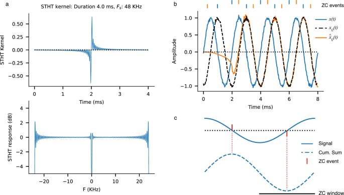
a The STHT kernel (top) which estimates the quadrature component x_Q of a signal, and frequency response of the kernel (bottom). b A noisy narrowband input signal (x; blue), with the quadrature component obtained from an infinite-time Hilbert transform (x_Q; dashed) and the STHT-derived version (({hat{x}}_{Q}); orange). Note the onset transient response of the filter before and around t < 2 ms. Corresponding up- and down-zero crossing encoding events estimated from x and ({hat{x}}_{Q}) are shown at top. c For a given signal (solid), zero crossings events (red) are estimated robustly by finding the peaks and troughs of the cumulative sum (dashed), within a window (ZC window).

Full size image

Secondly, infinite-time power integration likewise does not lend itself to streaming operation. The traditional solution is to average signal energy over a sliding window and update the estimate of the DoA periodically. Our proposed method instead performs low-pass filtering in the synapses and membranes of a spiking neural network, performing the time-averaging operation natively.

The STHT was computed by applying a convolutional kernel h[n] over a short window of length N to obtain an estimation of the Quadrature component x_Q[n] of a signal x[n]²⁸. To compute the kernel h[n], we made use of the linear property of the Hilbert transform (see Methods). Briefly, the impulse response of h[n] was obtained by applying the infinite-time Hilbert transform to the windowed Dirac delta signal δ_W[n] of length W, where δ_W[0] = 1 and δ_W[n] = 0 for n ≠ 0 and where W denotes the window length, and setting (h[n]={{{rm{Im}}}}left[{{{bf{H}}}}left[{delta }_{W}right]right][n]), where H is the Hilbert transform and ({{{rm{Im}}}}[cdot ]) is the imaginary part of the argument.

The STHT kernel for a duration of 4 ms is shown in Fig. 2a (top). The frequency response of this kernel (Fig. 2a, bottom) shows a predominately flat spectrum, with non-insignificant fluctuations for only low and high frequencies. The frequency width of this fluctuation area scales proportionally to the inverse of the duration of the kernel and can be chosen as needed by changing the kernel length W. In practice a bandpass filter should be applied to the audio signal before performing the STHT operation, to eliminate any distortions to low- and high-frequencies.

Figure 2 b illustrates the STHT applied to a noisy narrowband signal x(t) (blue; in-phase component). Following an onset transient due to the filtering settling time, the estimated STHT quadrature component ({hat{x}}_{{{{rm{Q}}}}}(t)) (orange) corresponds very closely to the infinite-time Hilbert transformed version x_Q(t) = H[x(t)] (dashed).

Robust Zero-crossing spike encoding

In order to perform the beamforming operation, we require an accurate estimation of the phase of the analytic signal. We chose to use SNNs to implement low-power, real-time estimation of DoA; this requires an event-based encoding of the audio signals for SNN processing. We propose an encoding method which robustly extracts and encodes the phase of the analytic signals, “Robust Zero-Crossing Conjugate” (RZCC) encoding. We estimated the zero crossings of a given signal by finding the peaks or troughs of the cumulative sum (Fig. 2c). Our approach generates both up- and down-going zero-crossing events. Each input signal channel therefore requires 2 or 4 event channels to encode the complex-valued analytic signal, depending on whether bi-polar or uni-polar zero crossing events are used. The events produced accurately encoded the phase of the in-phase and quadrature components of a noisy signal (Fig. 2b; top). Earlier works have used zero-crossing spike encoders to capture the phase of narrowband signals¹⁶. Our approach retains the phase of the full analytic signal, and is designed to operate robustly on wideband signals.

SNN-based implementation of Hilbert beamforming and DoA estimation

We implemented our Hilbert beamforming and DoA estimation approach in a simulated SNN (Fig. 3). We took the approach illustrated in Fig. 1d. We applied the STHT with kernel duration 10 ms, then used uni-polar RZCC encoding to obtain 2M event channels for the microphone array. In place of a complex-valued analytic signal, we concatenated the in-phase and quadrature components of the M signals to obtain 2M real-valued event channels.

a The pipeline for SNN implementation of our Hilbert beamforming and DoA estimation, combining Short-Time Hilbert transform; Zero-crossing conjugate encoding; analytically-derived beamforming weights; and Leaky-Integrate-and-Fire (LIF) spiking neurons for power accumulation and DoA estimation. b, c Beam patterns for SNN STHT RZCC beamforming, for narrowband (b; F = 2 kHz) and wideband (c; F_C = 2 kHz) signals. d, e Beam power and DoA estimates for noisy narrowband signals (d) and for noisy encoded speech (e). Dashed lines: estimated DoA. f, g DoA estimation error for noisy narrowband signals (f) and noisy speech (g). Dashed line: 1°. Annotations: Mean Absolute Error (MAE). Box plot: centre line: median; box limits: quartiles; whiskers: 1.5 × inter-quartile range; points: outliers. n = 100 random trials.

Full size image

Without loss of generality, our SNN implementation used Leaky Integrate-and-Fire neurons (LIF; see Methods). We chose synaptic and membrane time constants τ_s = τ_m = τ, such that the equivalent low-pass filter had a 3 dB corner frequency f_3 dB equal to the centre frequency of a signal of interest f (i.e. τ = 1/(2πf)).

We designed the SNN beamforming weights by simulating a template signal at a chosen DoA θ arriving at the array, and obtaining the resulting LIF membrane potentials r_x,θ(t), which is a 2M real-valued signal. When designing beamforming weights we neglected the effect of membrane reset on the membrane potential, assuming linearity in the neuron response. Concretely we used a chirp signal spanning 1.5–2.5 kHz as a template. We computed the beamforming weights by computing the sample covariance matrix ({hat{{{{bf{C}}}}}}_{x,theta }={{{rm{E}}}}{left[{{{{bf{r}}}}}_{x,theta }(t){{{{bf{r}}}}}_{x,theta }{(t)}^{{mathsf{T}}}right]}_{t}), where E[⋅]_t is the expectation over time. The beamforming weights are given by the SVD of ({hat{{{{bf{C}}}}}}_{x,theta }).

We reshaped the M-dimensioned complex signal into a 2M-dimensioned real-valued signal, by separating real and complex components. By doing so we therefore worked with the 2M × 2M real-valued covariance matrix. Due to the phase-shifted structure relating the in-phase and quadrature components of the analytic signal, the beamforming vectors obtained by PSD from the 2M × 2M covariance matrix are identical to those obtained from the M × M complex covariance matrix (See Supplementary Note 8).

Figure 3a–b shows the beam patterns for SNN Hilbert beamforming for narrowband (a) and wideband (b) signals (c.f. Fig. 1f–g). For narrowband signals, synchronization and regularity in the event encoded input resulted in worse resolution than for wideband signals. For noisy narrowband and noisy speech signals, beam patterns maintained good shape above 0 dB SNR (Fig. 3d–e).

We implemented DoA estimation using SNN Hilbert beamforming, and measured the estimation error on noisy narrowband signals (Fig. 3f–g). For SNR  > 10 dB we obtained an empirical Mean Absolute Error (MAE) of DoA estimation 1.08° on noisy narrowband signals (Fig. 3f). DoA error increased with lower SNR, with DoA error of approx 2.0° maintained for SNRs of -1 dB and higher. DoA error was considerably lower for noisy speech (Librispeech corpus²⁹; Fig. 3g), with DoA errors down to 0.29°.

We deployed DoA estimation using SNN Hilbert beamforming on a seven-microphone circular array (Fig. 1a) on live audio. A sound source was placed 1.5 m from the centre of the array, in a quiet office room with no particular acoustic preparation. We collected SNN output events with the peak event rate over G output channels in each 400 ms bin indicating the instantaneous DoA. A stable DoA estimation was obtained by computing the running median over 10 s (see Methods). We examined frequency bands between 1.6–2.6 kHz, and obtained a measured MAE of 0.25–0.65°.

These results are an advance on previous implementations of binaural and microphone-array source localization with SNNs. Wall et al. implemented a biologically-inspired SNN for binaural DoA estimation, comparing against a cross-correlation approach¹³. They obtained an MAE of 3.8° with their SNN, and 4.75° using a cross-correlation approach, both on narrowband signals. Escudero et al. implemented a biologically-inspired model of sound source localization using a neuromorphic audio encoding device¹⁴. They obtained an MAE of 2.32° on pure narrowband signals, and 3.4° on noisy narrowband signals. Ghosh et al. implemented a trained feed-forward SNN for binaural DoA estimation, obtaining an MAE of 2.6° on narrowband signals³⁰. Roozbehi et al. implemented a trained recurrent SNN for binaural DoA and distance estimation, obtaining an MAE of 3.4° on wideband signals³¹. Pan et al. implemented a trained recurrent SNN for DOA estimation on a circular microphone array³². They reported an MAE of 1.14° under SNR 20 dB traffic noise, and MAE of 1.02° in noise-free conditions³² (see Table 1).

We therefore set a state-of-the-art for SNN-based DoA estimation.

Deployment of DoA estimation to SNN hardware

We deployed our approach to the SNN inference architecture Xylo²⁷. Xylo implements a synchronous digital, low-bit-depth integer-logic hardware simulation of LIF spiking neurons. The Rockpool software toolchain³³ includes a bit-accurate simulation of the Xylo architecture, including quantization of parameters and training SNNs for deployment to Xylo-family hardware. We quantized and simulated the Hilbert SNN DoA estimation approach on the Xylo architecture, using bipolar RZCC spike encoding.

Global weight and LIF parameter quantization was performed by obtaining the maximum absolute beamforming weight value, then scaling the weights globally to ensure this maximum weight value mapped to 128, then rounding to the nearest integer. This ensured that all beamforming weights spanned the range −128 to 128.

Spike-based DoA estimation results are shown in Figure S9 and Table 1. For noisy speech we obtained a minimum MAE of 2.96° at SNR 14 dB.

We deployed a version of Hilbert SNN DoA estimation based on unipolar RZCC encoding to the XyloAudio 2 device^26,27. This is a resource-constrained low-power inference processor, supporting 16 input channels, up to 1000 spiking LIF hidden neurons, and 8 output channels. We used 2 × 7 input channels for unipolar RZCC-encoded analytic signals from the M = 7 microphone array channels, and with DoA estimation resolution of G = 449 as before. We implemented beamforming by deploying the quantized beamforming weights W (14 × 449) to the hidden layer on Xylo. We read out the spiking activity of 449 hidden layer neurons, and chose the DoA as the neuron with highest firing rate (({{{rm{arg,max}}}})). We measured continuous-time inference power on the Xylo processor while performing DoA estimation.

Note that the Xylo development device was not designed to provide the high master clock frequencies required for real-time operation for beamforming. Inference results were therefore slower than real-time on the development platform. This is not a limitation of the Xylo architecture, which could be customized to support real-time operation for beamforming and DoA estimation. When operated at 50 MHz, Xylo required 4.03 s to process 2.0 s of audio data, using 1139 μW total continuous inference power. With an efficient implementation of signed RZCC input spikes and weight sharing, the bipolar version would require an additional 10% of power consumption. In the worst case, the bipolar RZCC version would require double the power required for the unipolar version. Scaling our power measurements up for real-time bipolar RZCC operation, the Xylo architecture would perform continuous DoA estimation with 2.53–4.60 mW total inference power.

MUSIC beamforming

For comparison with our method, we implemented MUSIC beamforming for DoA estimation⁴, using an identical microphone array geometry. MUSIC is a narrowband beamforming approach, following the principles in Fig. 1b. Beam patterns for MUSIC on the same circular array are shown in Supplementary Fig. S6. Supplementary Fig. S5 shows the accuracy distribution for MUSIC DoA estimation (same conventions as Fig. 3d). For SNR 20 dB we obtained an empirical MAE for MUSIC of 1.53° on noisy narrowband signals, and MAE of 0.22° on noisy speech.

To estimate the first-stage power consumption of the MUSIC beamforming method, we reviewed recent methods for low-power Fast Fourier Transform (FFT) spectrum estimation. Recent work proposed a 128-point streaming FFT for six-channel audio in low-power 65 nm CMOS technology, with a power supply of 1.0 V and clock rate of 80 MHz³⁴. Another efficient implementation for 256-point FFT was reported for 65 nm CMOS, using a 1.2 V power supply and a clock rate of 877 MHz³⁵. To support a direct comparison with our method, we adjusted the reported results to align with the number of required FFT points, the CMOS technology node, the supply voltage and the master clock frequency used in Xylo (see Methods). After appropriate scaling, we estimate these FFT methods to require 149 mW and 18.37 mW respectively^34,35. These MUSIC power estimates include only FFT calculation and not beamforming or DoA estimation, and therefore reflect a lower bound for power consumption for MUSIC.

Resources required for DoA estimation

We compared the DoA estimation errors and resources required for Hilbert SNN beamforming (this work), multi-channel RSNN-based beamforming³² and MUSIC beamforming⁴ (Table 1). We estimated the compute resources required by each approach, by counting the memory cells used by each method. We did not take into account differences in implementing multiply-accumulate operations, or the computational requirements for implementing FFT filtering operations in the RSNN³² or MUSIC⁴ methods.

The previous state of the art for SNN beamforming and DoA estimation from a microphone array used a recurrent SNN to perform beamforming³². Their approach used a dense filterbank to obtain narrowband signal components, and a trained recurrent network with N_r = 1024 neurons for beamforming and DoA estimation. Their network architecture required input weights of CN_r from the C filterbank channels; ({N}_{{{{rm{r}}}}}^{2}) recurrent weights for the SNN; and N_rG output weights for the G DoA estimation channels. They also required N_r + G neuron states for their network. For the implementation described in their work, they required 1463712 memory cells for beamforming and DoA estimation.

The MUSIC beamforming approach uses a dense filterbank to obtain narrowband signals, and then weights and combines these to perform beamforming⁴. This approach requires CMG memory cells. For the implementation of MUSIC described here, 2514400 memory cells were required.

Since our Hilbert beamforming approach operates directly on wideband signals, we do not require a separate set of beamforming weights for each narrowband component of a source signal. In addition, we observed that the beamforming weights for down-going RZCC input events are simply a negative version of the beamforming weights for up-going RZCC input events (see Supplementary Note 7). This observation suggests an efficient implementation that includes signed event encoding of the analytic signal, in the RZCC event encoding block. This would permit a single set of beamforming weights to be reused, using the sign of the input event to effectively invert the sign of the beamforming weights. This approach would further halve the required resources for our DoA estimation method. Our method therefore requires 2MG memory cells to hold beamforming weights, and 2G neuron states for the LIF neurons. For the implementation described here, our approach required 7184 memory cells for beamforming and DoA estimation.

In the case of the quantized integer low-power architecture Xylo, the memory requirements are reduced further due to use of 8-bit weights and 16-bit neuron state.

Our Hilbert beamforming approach achieved very good accuracy under noisy conditions, using considerably lower compute resources than other approaches, and a fraction of the power required by traditional FFT-based beamforming methods.

Previous methods for beamforming and source separation using the Hilbert Transform

Several prior works performed source localization by estimating the time delay between arrival at multiple microphones. Kwak et al.³⁶ applied the Hilbert transform to obtain the signal envelope, then used cross-correlation between channels to estimate the delay. Several other works also obtained the Hilbert signal envelope and used the first peak of the amplitude envelope to estimate the delay from a sound event to a microphone in an array^37,38,39,40. These are not beamforming techniques, and make no use of the phase (or full analytic signal) for source localization.

Molla et al. applied the Hilbert transform after performing narrowband component estimation, to estimate instantaneous frequency and amplitude of incident audio⁴¹. They then estimated inter-aural time- and level- differences (ITD and ILD), and performed standard binaural source localization based on these values, without beamforming.

Kim et al. used the Hilbert transform to obtain a version of a high-frequency input signal which was decimated to reduce the complexity of a subsequent FFT⁴². They then performed traditional frequency-domain beamforming using the narrowband signals obtained through FFT. This is therefore distinct from our direct wideband beamforming approach.

Some works performed active beamforming on known signals, using the Hilbert transform to estimate per-channel delays prior to beamforming.^28,43 In these works, the Hilbert transform was used to obtain higher accuracy estimation of delays, where the transmitted signal is known. We instead use the increasing phase property of the Hilbert transform to provide a general beamforming approach applicable to unknown wideband and narrowband signals.

We introduced a beamforming approach for microphone arrays, suitable for implementation in a spiking neural network (SNN). We applied our approach to a direction-of-arrival (DoA) estimation task for far-field audio. Our method is based on the Hilbert transform, coupled with efficient zero-crossing based encoding of the analytic signal to preserve phase information. We showed that the phase of the analytic signal provides sufficient information to perform DoA estimation on wide-band signals, without requiring resource-intensive FFT or filterbank pre-processing to obtain narrow-band components. We provided an efficient implementation of our method in an SNN architecture targeting low-power deployment (Xylo²⁷). By comparing our approach with existing implementations of beamforming and DoA estimation for both classical and SNN architectures, we showed that our method obtains highly accurate DoA estimation for both noisy wideband signals and noisy speech, without requiring energy- and computationally-intensive filterbank preprocessing.

Our Hilbert beamforming approach allows us to apply a unified beamforming method for both narrowband and wideband signals. In particular, we do not need to decompose the incident signals into many narrowband components using an FFT or filterbank. This simplifies preprocessing and reduces resources and power consumption.

Our design for event-based zero-crossing input encoding (RZCC) suggests an architecture with signed input event channels (i.e.  +1, −1). The negative symmetric structure of the up-going and down-going RZCC channel Hilbert beamforming weights permits weight sharing over the signed input channels, allowing us to consider a highly resource- and power-efficient SNN architecture for deployment.

A key feature of our audio spike encoding method is to make use of the Hilbert analytic signal, making use of not only the in-phase component (i.e. the original input signal) but also the quadrature component, for spike encoding. Previous approaches for SNN-based beamforming used a dense narrowband filterbank, obtaining almost sinusoidal signals from which the quadrature spikes are directly predicable from in-phase spikes. Existing SNN implementations required considerably more complex network architectures for DoA estimation⁴⁴, perhaps explained by the need to first estimate quadrature events from in-phase events, and then combine estimations across multiple frequency bands. Our richer audio event encoding based on the STHT permits us to use a very simple network architecture for DoA estimation, and to operate directly on wideband signals.

While our approach permits unipolar RZCC event encoding and beamforming (i.e. using only up- or down-going events but not both), we observed bipolar RZCC event encoding was required to achieve high accuracy in DoA estimation. This increases the complexity of input handling slightly, requiring 2-bit signed input events instead of 1-bit unsigned events. The majority of SNN inference chips assume unsigned events, implying that modifications to existing hardware designs are required to deploy our method with full efficiency.

We showed that our approach achieves good DoA estimation accuracy on noisy wideband signals and noisy speech. In practice, if a frequency band of interest is known, it may be possible to achieve even better performance by first using a wide band-pass filter to limit the input audio to a wide band of interest.

We demonstrated that engineering an SNN-based solution from first principles can achieve very high accuracy for signal processing tasks, comparable with off-the-shelf methods designed for DSPs, and state-of-the-art for SNN approaches. Our approach is highly appropriate for ultra-low-power SNN inference processors, and shows that SNN solutions can compete with traditional computing methods without sacrificing performance.

Here we have demonstrated our method on a circular microphone array, but it applies equally well to alternative array geometries such as linear or random arrays with good performance (see Supplementary Figs. S7 and S8).

Our Hilbert Transform-based beamforming method can also be applied to DSP-based signal processing solutions, by using the analytical signal without RZCC event encoding (see Fig. 1f–g; Supplementary Fig. S6a–b). This can improve the computational- and energy-efficiency of traditional methods, by avoiding the need for large FFT implementations.

Signal Model

We denote the incoming signal from M microphones by ({{{bf{X}}}}(t)={({x}_{1}(t),ldots ,{x}_{M}(t))}^{{mathsf{T}}}) where x_i(t) denotes the time-domain signal received from the ith microphone i ∈ [M]. We adopted a far-field scenario where the signal received from each audio source can be approximated with a planar wave with well-defined direction of arrival (DoA). Under this model, when an audio source at DoA θ transmits a signal a(t), the received signal at the microphone i is given by

where z_i(t) denotes the additive noise in microphone i, where α is the attenuation factor (same for all microphones), and where τ_i(θ) denotes the delay from the audio source to microphone i ∈ [M] which depends on the DoA θ. In the far-field scenario we assumed that the attenuation parameters from the audio source to all the microphones are equal, and drop them after normalization. We also assume that

where ({tau }_{0}=frac{D}{c}) with D denoting the distance of the audio source from the center of the array, where c ≈ 340 m/s is the speed of sound in the open air, where R is the radius of the array, and where θ_i denotes the angle of the microphone i in the circular array configuration as illustrated in Fig. 1a.

Wideband noise signals

Random wideband signals were generated using coloured noise. White noise traces were generated using iid samples from a Normal distribution: (x[n] sim {{{mathcal{N}}}}(0,1)), with a sampling frequency of 48 kHz. These traces were then filtered using a second-order Butterworth bandpass filter from the python module scipy.filter.

Noisy speech signals

We used speech samples from the Librispeech corpus²⁹. These were normalized in amplitude, and mixed with white noise to obtain a specified target SNR.

Beamforming for DoA Estimation

The common approach for beamforming and DoA estimation for wideband signals is to apply DFT-like or other filterbank-based transforms to decompose the input signal into a collection of narrowband components as

where ({{{mathcal{F}}}}={{f}_{1},{f}_{2},ldots ,{f}_{F}}) is a collection of (F=leftvert {{{mathcal{F}}}}rightvert) central frequencies to which the input signal is decomposed. Beamforming is then performed on the narrowband components as follows.

When the source signal is narrowband and in the extreme case a sinusoid (x(t)=Asin (2pi {f}_{0}t)) of frequency f₀, time-of-arrival to different microphones appear as a constant phase shift

at each microphone i ∈ M where this phase-shift depends on the DoA θ. By combining the M received signal x_i(t) with appropriate weights ({{{{bf{w}}}}}_{theta }:= {({w}_{1,theta },ldots ,{w}_{M,theta })}^{{mathsf{T}}}), one may steer the array beam toward a specific θ corresponding to the source DoA and obtain the beamformed signal

By performing this operation over a range of test DoAs (tilde{theta }), the incident DoA can be estimated by finding (tilde{theta }) which maximizes the power of the signal obtained after beamforming:

Hilbert beamforming

To generate beamforming vectors, we first choose a desired precision for DoA estimation by quantizing DoAs into a grid ({{{mathcal{G}}}}={{theta }_{1},ldots ,{theta }_{G}}) of size G where G = κM where κ > 1 denotes the spatial oversampling factor.

We choose a template representative for the audio signal x(t), apply the HT to obtain its analytic version x_a(t), compute ({hat{{{{bf{C}}}}}}_{x,g}) for each angle (gin {{{mathcal{G}}}}), and design beamforming vectors ({{{{mathcal{W}}}}}_{{{{mathcal{G}}}}}:= {{{{{bf{w}}}}}_{g}:gin G}). We arrange the beamforming vectors as an M × G beamforming matrix W = [w₀, …, w_G−1]. In practice we choose a chirp signal for x(t), spanning 1–3 kHz.

We estimate the DoA of a target signal as follows. We receive the M-dim time-domain signal X(t) incident to the microphone array over a time-interval of duration T and apply the STHT to obtain the analytic signal X_a(t).

We then apply beamforming using the matrix W to compute the G-dim time-domain beamformed signal

We accumulate the power of the beamformed signal X_b(t) over the whole interval T, and compute the average power over the grid elements as a G-dim vector ({{{bf{p}}}}={({p}_{1},ldots ,{p}_{G})}^{{mathsf{T}}}), where

Finally we estimate the DoA of a target by identifying the DoA in ({{{mathcal{G}}}}) corresponding to the maximum power, such that

DoA estimation with live audio

We recorded live audio using a 7-channel circular microphone array (UMA-8 v2, radius 45 mm), sampled at 48 kHz. The microphone array and sound source (speaker width approx. 6 mm) were placed in a quiet office environment with no particular acoustic preparation, separated by 1.5 m. We implemented Hilbert SNN beamforming, with G = 449 DoA bins, and a Hilbert kernel of 20 ms duration. Chirp signals were used for template signals when generating beamforming weights, with a duration of 400 ms and a frequency range of 1.6–2.6 kHz. Bipolar RZCC audio to event encoding was used. Output events were collected over the G output channels, and the channel with highest event rate in each 400 ms bin was taken to indicate the instantaneous DoA estimate. To produce a sample DoA estimation, windows of 10 s (25 bins) were collected, and the running median was computed over each window. This was taken as the final DoA estimate. Mean Absolute Error (MAE) was computed to measure the accuracy of DoA estimation.

LIF spiking neuron

We use an LIF (leaky integrate and fire) spiking neuron model (See Supplementary Fig. S4), in which impulse responses of synapse and neuron are given by ({h}_{s}(t)={e}^{-frac{t}{{tau }_{s}}}u(t)) and ({h}_{n}(t)={e}^{-frac{t}{{tau }_{n}}}u(t)), where τ_s and τ_n denote the time-constants of the synapse and neuron, respectively. LIF filters can be efficiently implemented by 1^st order filters and bitshift circuits in digital hardware. Here we set τ_s = τ_n = τ. For such a choice of parameters, the frequency response of the cascade of synapse and neuron is given by

which has a 3dB corner frequency of ({f}_{3{{{rm{dB}}}}}=frac{1}{2pi tau }).

MUSIC beamforming for DoA estimation

We compared our proposed method with the state-of-the-art super-resolution localization method based on the MUSIC algorithm. Our implementation of MUSIC proceeds as follows.

We apply a Fast Fourier Transform (FFT) to sequences of 50 ms audio segments, sampled at 48 kHz (N = 2400 samples), retaining only those frequency bins in the range 1.6–2.4 kHz. This configuration achieves an angular precision of 1° while minimizing power consumption and computational complexity. See Supplementary Note 8 for details on setting parameters for MUSIC.

We compute the array response matrix for the retained FFT frequencies to target an angular precision of 1°. To reduce the power consumption and computational complexity of MUSIC further, we retain only F = 1 FFT frequency bin for localization, thus requiring only a single beamforming matrix. Considering G = 225 angular bins (where G = 225 = 7 × 32 + 1, for a microphone array board with M = 7 microphones, thus, an angular oversampling factor of 32), each array response matrix will be of dimension 7 × 225.

MUSIC beamforming was performed by applying FFT to frames from each microphone, choosing the highest-power frequency bin in the range 1.6–2.4 kHz, and multiplying with the array response matrix for that freqeuncy. We then accumulated power over time for each DoA g ∈ G, to identify the DoA with maximum power as the estimated incident DoA.

To estimate power consumption for MUSIC, we performed a survey of recent works on hardware implementation of the MUSIC algorithm, where the FFT frame size, number of microphone channels, fabrication technology, rail voltage, clock speed and resulting power consumption were all reported. This allowed us to re-scale the reported power to match the required configuration of our MUSIC configuration, and to match the configuration of Xylo used in our own power estimates.

For example, in Ref. ³⁴ the authors implemented a 128-point FFT in streaming mode for a 6-channel input signal in 65 nm CMOS technology with a power supply of 1.0 V and clock rate of 80 MHz, achieving a power consumption of around 10.32 mW. Scaling the power to 40 nm technology and 1.1 V power supply on Xylo, assuming 7-channel input audio with a sampling rate of 48 kHz and FFT length N = 2048 for our proposed MUSIC implementation, yields a power consumption of

where the last two factors denote the effect of technology and power supply. We made the optimistic assumption that the power consumption in streaming mode grows only proportionally to FFT frame length. We included only power required by the initial FFT for MUSIC, and neglected the additional computational energy required for beamforming and DoA estimation itself. Our MUSIC power estimates are therefore a conservative lower bound.