Machine learning-guided integration of fixed and mobile sensors for high resolution urban PM2.5 mapping

Urban centers are densely populated areas where fine particulate matter (PM_2.5) pollution has been one of the primary environmental concerns since the 20th century. Prolonged exposure to severe PM_2.5 pollution poses substantial threats to human health, including increased risks of premature death^1,2. The emission sources in urban areas are diverse and unevenly distributed. Due to complex physical and chemical processes, PM_2.5 concentrations exhibit significant local variations over short distances and periods within urban environments^3,4,5. High spatiotemporal resolution air quality maps are crucial for capturing fine-scale pollution hotspots, reducing exposure measurement errors, and mitigating public health risks and environmental injustices^6,7. Moreover, understanding the causes of PM_2.5 pollution facilitates effective air quality management.

Traditionally, chemical transport model simulations^8,9,10, land use regression modeling¹¹, and satellite retrievals¹² have been extensively employed to track the dynamic fluctuations of air quality. However, these methods have inherent limitations when treated with fine-scale urban air pollution. Chemical transport models entail high computational costs and rely on frequent updates of emission inventories. Satellite data, although globally comprehensive, are hindered by issues such as cloud cover¹³. Land use regression models rely on fixed–location monitoring and geographic information system predictor variables, which are constrained by specific local administrative boundaries and often lack the precision required at larger geographic scales¹⁴. Additionally, sparse monitoring networks prove ineffective at capturing fine-scale pollution hotspots, resulting in inadequate depictions of spatiotemporal heterogeneity of urban air quality¹⁵. In recent years, advancements in low–cost sensor technology have improved the ability to monitor fine–scale concentration gradients^16,17,18,19. Nevertheless, challenges remain in achieving sufficient data frequency and statistical robustness for temporal representation^20,21. To effectively map urban air quality and comprehensively understand the spatiotemporal dynamics of air pollution, extensive data collection, and advanced statistical methods are essential.

Generally, intensive emission sources, unfavorable meteorological conditions, and plume transport are key factors that can lead to urban PM_2.5 pollution events^22,23,24,25. Thorough attribution analysis, utilizing advanced statistical methods, is essential for providing scientific support for regulatory strategies and effective urban air quality management. In recent years, machine learning (ML) has demonstrated remarkable promise in air quality modeling due to its exceptional ability to capture complex and nonlinear relationships between different variables^26,27,28. Compared to traditional methods, ML models can effectively integrate large amounts of multi-source heterogeneous data, such as meteorological, traffic, and geographical information, to make more accurate and real-time predictions of PM_2.5 pollution events. However, these models often face criticism for their “black–box” nature, which makes it difficult to understand the underlying factors driving their predictions. The development and integration of explainable artificial intelligence (XAI) techniques, such as Shapley additive explanations (SHAP), has become a crucial tool for providing transparency in ML models and elucidating the intricacies of air pollution^{29,30,31,32,33}. By quantifying the contributions of individual features, SHAP enables researchers and policymakers to identify key drivers of air pollution events, offering critical insights for crafting targeted mitigation strategies. This interpretability not only enhances the transparency of predictions but also builds trust among stakeholders, facilitating more informed decision–making to improve urban air quality and protect public health.

In this study, we focused on the mapping and attribution of PM_2.5 pollution in urban Jinan, the capital of a province located in the heavily polluted North China Plain. Utilizing a large–scale, low–cost mobile, and fixed sensor network combined with advanced machine learning algorithms for spatiotemporal modeling, we developed a novel method for generating high spatiotemporal resolution (500 m × 500 m and 1 h) PM_2.5 datasets. We then explored the optimal arrangement of mobile and fixed sensor monitoring to achieve continuous, high–precision monitoring while minimizing costs, providing valuable insights for urban air quality management. Finally, we accurately quantified the contributions of various factors to urban PM_2.5 pollution by coupling positive matrix factorization (PMF), the hybrid single-particle Lagrangian integrated trajectory (HYSPLIT), and SHAP, providing a scientific basis for accurately identifying the causes of air pollution and enabling precise control measures.

High spatiotemporal resolution PM_2.5 pollution mapping

Our dataset can effectively capture the hourly variations in PM_2.5 concentrations, which is valuable for mitigating the health impacts of acute exposure and facilitating environmental management. Taking a typical severe PM_2.5 pollution event during February 5 and 6, 2019 (the Spring Festival) in urban Jinan as an example (Fig. 1), our dataset nearly perfectly captured the entire evolution of air quality from clean conditions to severe pollution and subsequent dispersion. From 0:00 to 17:00 (local time) on February 5, data from the atmospheric supersite indicated an hourly average PM_{2.5_as} concentration of 68 ± 24 μg/m³. Starting at 18:00, PM_2.5 pollution began to encroach upon the urban area from the north, initially manifesting as localized contamination. By 0:00 on February 6, severe pollution had enveloped most urban areas, with PM_2.5 concentrations at the atmospheric supersite peaking at 198 ± 84 μg/m³. Subsequently, the pollution gradually dissipated as north and northwest winds persisted. This pattern aligns with the occurrence of northwest winds after 23:00 on February 5, as reported by timeanddate (https://www.timeanddate.com/weather/china/jinan/historic?month=2&year=2019). The six China National Environmental Monitoring Center sites within the urban area and Jinan atmospheric supersite also documented fluctuations in PM_2.5 concentrations throughout the pollution formation and dispersion process between February 5 and 6. These observations are consistent with the spatiotemporal PM_2.5 pollution mapping results generated by our air quality inference model, as depicted in Supplementary Fig. 1.

The selected period of February 5 and 6, 2019, highlights the spatiotemporal dynamics of PM_2.5 concentrations in the 900 km² study area of Jinan, with a 500 m spatial resolution and 1 h temporal resolution.

Full size image

Evaluation of mapping before and after reducing fixed micro-stations

Using the same methodology described in the fourth part of “Methods” and integrating data from a reduced number of micro-fixed monitoring sites as outlined in the fifth part of “Methods”, we developed another set of PM_2.5 data products. This endeavor aims to explore different layouts for combining mobile and micro-fixed monitoring to achieve high-precision urban air quality monitoring while minimizing costs. Figure 2 compares the efficacy of datasets before and after reducing the number of micro-fixed sites on hourly, daily, and monthly scales. We selected a severe PM_2.5 pollution event on December 10, 2019, to evaluate the effectiveness of both datasets in capturing pollution processes on an hourly scale. By midnight on December 10, PM_2.5 pollution was severe in most areas of urban Jinan, particularly in the downtown core, with the exception of the southeastern urban area. By 7:00, PM_2.5 pollution in the downtown area had been alleviated.

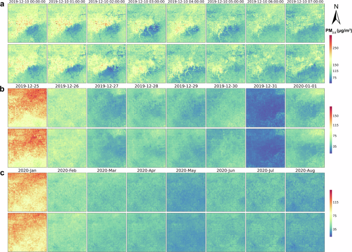
Comparative evaluation of mapping effects on a hourly scale, b daily scale, and c monthly scale before and after the reduction of micro-fixed monitoring points. The panels in the first, third, and fifth rows display the spatiotemporal distributions of hourly, daily, and monthly averages of PM_2.5 concentration data products developed from multi-source data before reducing the number of micro-fixed monitoring points. In contrast, the panels in the second, fourth, and sixth rows depict the corresponding distributions after the reduction.

Full size image

On the daily scale, we examined the period from December 25, 2019, to January 1, 2020, as a case study. According to our dataset, on December 25th, most areas exhibited pollution. Pollution gradually abated in the subsequent days, and by December 31st, most parts of the city had achieved clean air status. On the monthly scale, for instance, PM_2.5 concentrations in January 2020 exceeded that of other listed months in 2020. Seasonal analysis further reveals that winter air quality in Jinan is considerably poorer than in spring, summer, and autumn (Supplementary Fig. 2), likely driven by increased heating emissions and specific meteorological conditions that facilitate pollutant accumulation³⁴. Such seasonal disparities highlight winter-specific pollution challenges, underscoring the unique air quality management needs during this season. Overall, across hourly, daily, monthly, and seasonal scales, the patterns of PM_2.5 concentration variations align with urban area observations (Supplementary Figs. 3-6). Both sets of PM_2.5 data products effectively capture high-value areas and fine-scale dynamic changes in PM_2.5 concentrations within urban settings. These findings underscore the significant potential of integrating mobile and micro-fixed monitoring to develop high spatiotemporal PM_2.5 concentration datasets. Moreover, the dataset built after selectively reducing fixed micro-stations has shown promising results. This outcome not only significantly reduces government expenditures but also holds crucial implications for optimizing the spatial distribution of mobile and fixed micro–station monitoring to enhance the development of high–resolution spatiotemporal datasets.

Key drivers and interpretability attribution of PM_2.5 in Jinan

Figure 3a displays the driving factors influencing PM_2.5 concentrations in Jinan, ranked by mean absolute SHAP values. SIA exhibited the highest importance, with an absolute SHAP mean value of 15.83, significantly surpassing other features such as IP (5.70), BB (5.32), T_as (4.57), and Dust (3.78). These five drivers predominantly influenced PM_2.5 concentrations from January 2019 to September 2021. AOD and BLH made comparable contributions, with values ranging from 3 to 3.4, while RH_as (2.85) and P (2.52) had slightly weaker impacts. Ox (1.93) played a significant role due to increased radiation and temperature at noon, enhancing photochemical processes³⁵. Primary emission sources like CC (1.90) and VE (1.78) contributed less to PM_2.5 compared to IP, BB, and Dust. Cluster, SSR, WS_as, TCC, and WD_as had relatively minor predictive effects.

The impacts of driving factors on PM_2.5 concentration in Jinan from January 2019 to September 2021. (a) Mean absolute SHAP values of various drivers on PM_2.5 concentration. (b) Responses of SHAP values to the top twelve important predictors for PM_2.5. Panels are shown as joint plots, where colors in the main plot indicate sample density (dark blue represents high density), with marginal plots showing the distributions of predictor (top) and response (right). SIA: secondary inorganic aerosol; IP: industrial pollution; BB: biomass burning; T: T_as, temperature; Dust: dust emission; AOD: aerosol optical depth; BLH: boundary layer height; RH: RH_as, relative humidity; P: pressure; O_X: total gaseous oxidant (NO₂ + O₃); CC: coal combustion; VE: vehicle emissions; Cluster: air mass trajectory; SSR: surface net solar radiation; WS: WS_as, wind speed; TCC: total cloud cover; WD: WD_as, wind direction. For more information, see the Methods section.

Full size image

Figure 3b illustrates the response between measured or proxy values of factors and their corresponding SHAP values with respect to PM_2.5 concentrations, offering additional insights into each factor’s influence. Factors such as SIA, IP, BB, and other emission sources showed a pronounced positive contribution to PM_2.5, highlighting the substantial impact of both secondary formation and primary emissions on air quality in Jinan. Similar positive effects were also observed for AOD, RH_as, and O_X. Notably, RH_as positively contributed to PM_2.5 when exceeded 60%, enhancing its formation through aqueous–phase chemistry and hygroscopic growth^29,36,37. Conversely, P, T_as, and BLH exhibited a negative relationship with PM_2.5 concentrations. Low-pressure systems, usually associated with high humidity, can synergistically enhance PM_2.5 condensation and coagulation, leading to elevated concentrations^38,39. Previous literatures have also reported negative effects of atmospheric pressure on PM_2.5 concentrations in places like Beijing⁴⁰ and Hangzhou³⁹. A low BLH restricts horizontal and vertical transport, increasing near-surface humidity⁴¹. High humidity, in turn, enhances aerosol hygroscopic growth, amplifying the positive feedback between aerosols and the boundary layer. This feedback may intensify cross-boundary air pollution transport, exacerbating continuous PM_2.5 generation^8,42. Our findings show that SHAP values for air masses 1 and 7 were positive, while air masses 2, 3, and 6 negatively impacted PM_2.5 concentrations (Supplementary Fig. 7). This suggests that pollutants transported from border areas between northern Zibo and southeastern Binzhou in Shandong, as well as northern Henan and southern Shanxi (Supplementary Fig. 8), increased PM_2.5 concentrations in Jinan. Conversely, air masses from Mongolia and northeastern Inner Mongolia typically exhibited a cleansing effect. The breakdown in Supplementary Figs. 9 and 10 further delineates the seasonal and pollution-level-specific contributions of various factors to PM_2.5 concentrations. Seasonal shifts highlight SIA, IP, and BB as key contributors. As PM_2.5 concentrations rise, emissions from pollution sources and lowered BLH amplify concentrations. Moreover, the impacts of driving factors on the diurnal and nocturnal mechanisms of PM_2.5 formation are summarized in Fig. 4 and Supplementary Fig. 11.

Pink and blue arrows denote variations in measured values for each driver and their respective impacts on PM_2.5 concentrations. The diurnal influences of P and BLH influencing PM_2.5 concentrations are not observed, and hence, they are depicted in the light orange shaded area centrally in the figure. Relevant calculations are derived from Supplementary Fig. 11.

Full size image

In this study, we employed an advanced light gradient boosting machine (LightGBM), a gradient boosting framework developed by a research team at Microsoft Research Asia⁴³, to conduct multi-objective model simulations. LightGBM offers lower memory consumption and faster training speed, making it especially suitable for large-scale data analysis, and has demonstrated effective applicability in related studies^44,45,46,47. To validate the performance of LightGBM, we compared it with XGBoost and Random Forest (RF) using 70% and 80% training data splits and various hyperparameter settings. Results in Supplementary Tables 1–3 show that LightGBM consistently outperforms XGBoost and RF, demonstrating robust performance on large datasets. LightGBM’s histogram-based decision tree algorithm, which bins continuous features, enables faster node splitting and lower memory usage. In contrast, XGBoost performs precise but computationally intensive splits, while RF requires each tree to be trained independently, increasing resource demands. Additionally, leaf-wise growth and efficient parallelism make LightGBM better suited for data-intensive tasks. Notably, for large datasets, a 70% training set yielded similar or better results than 80%, as more data added minimal benefit while increasing computational costs. The computational efficiency of LightGBM makes it highly applicable to the vast and growing atmospheric environmental datasets. Prioritizing LightGBM in future applications will help meet the demand for high–accuracy, real-time environmental modeling and analysis.

Our study demonstrates that combining mobile and micro-fixed monitoring enables high-resolution air quality monitoring in urban areas, effectively capturing the spatial heterogeneity of PM_2.5 concentrations. This approach aligns with the needs of policymakers and urban planners who require detailed pollution mapping to make targeted interventions. For example, the ability to dynamically monitor pollution hotspots can inform the timely allocation of resources, such as deploying temporary traffic restrictions or emission reduction measures in critical areas. Furthermore, our optimization of micro-fixed monitoring sites has demonstrated that integrating mobile monitoring maintains coverage while potentially reducing monitoring costs by nearly 70%, from 612 to 184 micro-fixed sites. This reduction illustrates a practical path for cities with limited budgets to still achieve robust air quality monitoring. Additionally, with future research, we aim to evaluate alternative configurations of monitoring networks, such as exploring the effects of different fleet sizes and variations in micro-fixed site density. By assessing these factors, it may be possible to optimize the network further to reduce costs or enhance coverage without sacrificing data quality. These findings can provide a concrete basis for policy recommendations on network design, resource allocation, and budget optimization in urban air quality monitoring frameworks. However, the high data volume and computational intensity of our approach underscore the need for efficient data processing infrastructures that can provide actionable, real-time insights to urban planners and policymakers. Our results suggest that strategic reductions in both mobile and micro–fixed monitoring densities may be feasible, enabling more flexible deployment models that balance cost, resource allocation, and monitoring effectiveness. This approach ultimately supports more accessible and economically viable air quality management solutions for urban areas.

Our proposed PMF-HYSPLIT-LightGBM-SHAP coupled model provides a tool for quantifying the contributions of sources, meteorology, and regional transport to PM_2.5 concentrations, and holds significant potential and value in analyzing the causes of PM_2.5 pollution. However, due to data limitations, certain constraints still exist. The formation of PM_2.5 is also influenced by other factors, such as “doming effect” of black carbon⁴⁸ and chemical interactions among volatile organic compounds, Ozone (O₃), and PM_2.5. Further evaluation of their impacts on PM_2.5 is necessary.

In summary, we propose an innovative method for developing high–resolution spatiotemporal maps of urban PM_2.5 using mobile and micro-fixed monitoring networks, which can capture fine-scale PM_2.5 spatial heterogeneity within the urban area. This method not only advances the precision of air quality assessments but also provides valuable insights for optimizing the deployment of mobile and micro-sensor networks, offering significant economic benefits and reference value for deploying monitoring networks in other cities across China and potentially worldwide. Furthermore, by integrating XAI with existing atmospheric models, our research introduces a novel framework for understanding and attributing PM_2.5 sources, enhancing the depth of analysis and supporting more informed air quality management strategies. Incorporating real-time data into our PMF-HYSPLIT-LightGBM-SHAP coupled model could enhance its dynamic, real-world monitoring capabilities. Integrating continuous measurements from urban monitoring stations, GPS-based traffic data, meteorological inputs, and other diverse data sources through API-based data transfer could enable real-time predictions and model adjustments, providing immediate insights into PM_2.5 levels. Techniques such as scheduled updates or incremental learning could maintain model stability and accuracy amid continuous data flow. Although real-time monitoring presents challenges, including data latency, quality variability, and processing demands, addressing these could significantly enhance the model’s practical utility for quick source identification and adaptive responses to pollution events. Future research will address these technical challenges to further optimize the model for dynamic monitoring scenarios. Looking ahead, we will also focus on refining these models to improve predictive capabilities, expanding the application of our approach to diverse urban environments, and integrating real-time data to dynamically inform and adapt air quality interventions.

The methodological framework of the study

Figure 5 presents a schematic of the entire build process for this study, illustrating the data sources, machine learning model construction processes, and statistical methods utilized in the analysis. Three models were evaluated: LightGBM, XGBoost, and RF, considering different training data sizes and hyperparameter combinations. The coefficient of determination (R²), root mean square error (RMSE), and mean absolute error (MAE) were used as criteria to assess model performance. A description of three performance metrics can be found in Supplementary Text 1. More information about the three model settings can be found in Supplementary Text 2. Based on the comparative results (Supplementary Tables 1–3), a 70% training data split was selected, and the highest-performing LightGBM model was chosen to conduct high spatiotemporal resolution PM_2.5 mapping and pollution attribution analysis.

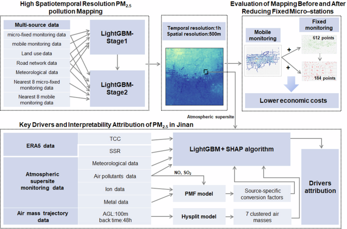
The methodological framework includes three main components: high spatiotemporal resolution PM_2.5 pollution mapping, evaluation of mapping before and after reducing fixed micro-stations, and key drivers and interpretability attribution of PM_2.5 in Jinan.

Full size image

Study area

Jinan, the provincial capital of Shandong Province, with a population exceeding 8 million and over 3.4 million registered vehicles⁴⁹, exemplifies a city with a high level of motorization. Considering the operational scope of our pilot vehicles, this study primarily focuses on the urban districts of Jinan (Supplementary Fig. 12). This area spans 900 km², is characterized by high population density, and serves as the core region for transportation, administration, commerce, and residential activities in Jinan. This work utilizes nearly three years of continuous air quality data collected from January 1, 2019, to September 13, 2021, through mobile cruising monitoring with vehicle-based sensors and fixed–location monitoring with micro–stations in the study area.

Source of the data

In the context of urban air quality inference and pollution attribution analysis, PM_2.5 concentrations within a given grid may be influenced by various local factors such as land use characteristics and traffic road networks, as well as external factors, including meteorological information. These factors collectively impact the emission and diffusion of local pollutants and the transport of regional pollutants. Therefore, the collected data comprises seven distinct components: mobile monitoring data (PM_{2.5_mobile}), fixed micro-station monitoring data (PM_{2.5_micro-fixed}, Wind speed_micro-fixed, Wind direction_micro-fixed, Relative humidity_micro-fixed, Temperature_micro-fixed), atmospheric supersite (36.67° N, 117.17°E) data (PM_{2.5_as}, SO₂, NO–NO₂–NO_X, O₃, Wind speed_as (WS_as), Wind direction_as (WD_as), Relative humidity_as (RH_as), Temperature_as (T_as), Pressure (P), Aerosol Optical Depth (AOD), Boundary Layer Height (BLH), SO₄²⁻, NH₄⁺, NO₃⁻, K, Ca, Mn, Zn, Fe, Pb), China National Environmental Monitoring Center (CNEMC) data (PM_{2.5_cnemc}), land use data, road network data, air mass trajectory data, and European Center for Medium-Range Weather Forecasts Reanalysis v5 (ERA5) data (Total cloud cover (TCC), Surface net solar radiation (SSR)). The mobile and fixed micro–station monitoring devices are equipped with four independent particle monitoring sensors that operate synchronously, cross-verify data with each other. In the event of a sensor malfunction, the other sensors continue to function normally, ensuring maximum data reliability. All data were either measured in the field or are publicly available. Detailed information about these multi-source data can be found in Supplementary Table 4.

PM_2.5 concentration inference model construction

A total of 612 fixed micro-station monitoring are unevenly distributed across 3600 grids in the study area, resulting in many grids lacking continuous monitoring. To address this challenge, we combined multi-source data (mobile monitoring, fixed micro-station monitoring, meteorological, road network, and land use data) to build two-stage LightGBM models to achieve full–coverage continuous monitoring with 500 m × 500 m spatial resolution and 1 h temporal resolution. First, we estimated hourly PM_2.5 concentrations based on multi-source data for grids with mobile monitoring data but no fixed micro-station data. These estimates served as proxies for the true ground-based fixed monitoring values in these grids. We then used these proxy values to estimate hourly PM_2.5 concentrations for grids lacking both mobile and fixed micro–station data, enabling high spatiotemporal resolution mapping of PM_2.5 concentrations across the entire study area.

Specifically, meteorological, road network, land use, mobile monitoring, and fixed micro-station monitoring data were allocated to grids. We used meteorological, land use, and mobile monitoring data from grids with both mobile and fixed micro-station monitoring data as input variables, while fixed micro-station data served as labels for constructing LightGBM_reconstruct-Stage1. Subsequently, this model estimated hourly PM_2.5 concentrations in grids with mobile monitoring data but without fixed micro-station data, with these estimates serving as proxies for ground-based fixed monitoring values. LightGBM_reconstruct-Stage2 was trained using the nearest spatially adjacent data points, including eight fixed micro-station observations, eight mobile observations, and meteorological, land use, and road network data from the same hour. These variables, along with PM_2.5 concentrations from grids equipped with fixed micro-station monitoring data, were used to predict hourly PM_2.5 concentrations in grids lacking both mobile and fixed micro-station monitoring data. Figure 5 and Supplementary Fig. 13 show schematic diagrams of the construction processes, while Supplementary Text 3 presents a more detailed description.

Both LightGBM_reconstruct models performed well on the testing set (Supplementary Fig. 14a, b), with R² of 0.91 for the first stage model (LightGBM_reconstruct-Stage1) and R² of 0.97 for the second stage model (LightGBM_reconstruct-Stage2), indicating that constructed models effectively infer PM_2.5 concentrations.

Inference model development based on new strategy

In an effort to optimize the budget while maintaining effective air quality monitoring, we divided the study area into 17 target regions as shown in Fig. 6. Following the algorithm outlined below, we selected the six nearest fixed micro-stations to the center point of each target region, ranging from target region 1 to target region 17. The specific algorithm formulas are as follows:

a The heatmap of mobile monitoring driving routes. b Original distribution of 612 micro-fixed monitoring sites. c The distribution of 184 micro-fixed monitoring sites retained using the new strategy.

Full size image

({Ln}{g}_{i}) and ({La}{t}_{i}) denote the longitude and latitude of fixed micro-stations in the target regions, respectively. Center_lon and Center_lat refer to the longitude and latitude of each target region’s center point. ({D}_{i}) represents the distance from each fixed micro-station to the center. (X) represents the set of distances from each fixed micro-station to the center point, and (N) signifies the number of the fixed micro-station in the target areas. Here, we defined the sorting operation function (S) and selection function (H). Therefore, ({H}_{6}) select the 6 fixed micro–stations closest to the center of each target region based on the smallest sorted distances.

Based on the above process, we selected 184 out of 612 fixed micro-stations and replicated the steps above-mentioned in the fourth part of “Methods” to train the LightGBM_strategy model for inferring PM_2.5 concentrations. Surprisingly, the two–stage LightGBM_strategy model still performed strongly, achieving R² values of 0.87 and 0.97, respectively (Supplementary Fig. 14c,d).

Development of PM_2.5 pollution attribution model

To identify key factors influencing PM_2.5 concentrations, we integrated the PMF model, HYSPLIT model, LightGBM model, and SHAP algorithm to establish an interpretable predictive model and elucidate each feature’s contribution. The main equation for SHAP is:

Here, (fleft({x}_{i}right)) represents the predicted value for each sample (left({x}_{i}right)) with (K) features and ({varphi }_{q}left(f,xright)) is the output expectation of the model for all samples, and ({varphi }_{p}left(f,{x}_{i}right)) denotes the Shapley value of feature (p) on the predicted outcome of the sample (left({x}_{i}right)). Detailed calculations are provided in Supplementary Text 4.

Initially, three species of water-soluble ions (NH₄⁺, NO₃⁻, SO₄²⁻), metal elements (K, Ca, Mn, Fe, Zn, Pb), and atmospheric pollutants (NO, SO₂) were selected for PMF analysis using US EPA PMF v5.0. We identified six sources: Coal Combustion (CC), Dust Emissions (Dust), Industrial Pollution (IP), Vehicular Emissions (VE), Biomass Burning (BB), and Secondary Inorganic Aerosol (SIA). Further details about PMF analysis can be found in Supplementary Text 5 and Supplementary Fig. 15. Subsequently, the HYSPLIT model was applied to calculate air clusters and characterize the air mass transport. For each hourly measurement, 48 h backward air mass trajectories at 100 m above ground level were calculated and clustered into seven groups (Supplementary Fig. 8). Total gaseous oxidant (O_X = NO₂ + O₃) served as a proxy for atmospheric photochemical oxidation conditions. We then input multiple variables including six emission sources (SIA, CC, BB, IP, Dust, VE), regional transport characteristics (Clusters), atmospheric oxidation condition (O_X), and meteorological parameters (BLH, WS_as, T_as, RH_as, AOD, TCC, SSR, P, WD_as) into the LightGBM_cause model to analyze PM_2.5 attribution. The LightGBM_cause model achieved strong performance with an R² of 0.89, RMSE of 14.18, and MAE of 8.93 (Supplementary Fig. 16), demonstrating an effective explanation of PM_2.5 concentration changes. Finally, we employed the SHAP algorithm as an XAI tool to quantify each feature’s contribution, thereby elucidating the factors contributing to PM_2.5 pollution in Jinan.