Magnetic memory and distinct spin populations in ferromagnetic Co3Sn2S2

First synthesized as a ternary chalcogenide with Shandite structure¹, Co₃Sn₂S₂ became a subject of tremendous attention after its identification as a ferromagnetic Weyl semi-metal^2,3. It crystallizes in a rhombohedral structure with ({rm{R}}bar{3}{rm{m}}) space group (n^∘166). The cobalt atoms form kagome sheets in the ab plane, which are separated by blocks of Sn and S atoms (see Fig. 1a). It magnetically orders below T_C ≈ 175 K with a saturation moment of ≈ 0.3 μ_B per Co atom⁴, and with the easy axis residing along the c-axis. Ab initio band calculations⁵, as well as photoemission⁶ and Mössbauer experiments⁷ identified it as a ferromagnetic half-metal. It is also a semi-metal with an equally low concentration of electrons and holes (n = p ≃ 8.7 × 10⁻¹⁹cm^{−3 8}). Thanks to such a low carrier density (comparable to elemental antimony, where n = p ≃ 6.6 × 10⁻¹⁹cm⁻³), mobility is sufficiently large to detect quantum oscillations and experimentally confirm the theoretically computed Fermi surface, consisting of two electron-like and two hole-like and multiply degenerate sheets⁹.

a Crystal structure of Co₃Sn₂S₂ with arrows showing the orientation of spins in the ordered phase. b Magnetization as a function of temperature at several magnetic fields. Above 22 mT, magnetization in the ferromagnetic phase is featureless. But when the sample is cooled down in presence of a magnetic field smaller than this threshold field, there is an anomaly and a hysteresis, which extends down to ≃110 K.

Full size image

The low carrier density implies that each mobile electron is shared by several hundred formula units of Co₃Sn₂S₂. This distinct feature leads to an exceptionally large anomalous Hall angle². Indeed, although the anomalous Hall conductivity of Co₃Sn₂S₂ (({sigma }_{xy}^{A})(2K) ≃ 1200(Ωcm)^{−1 2,8}) falls below what is seen in CoMn₂Ga (({sigma }_{xy}^{A})(2 K) ≃ 2000(Ωcm)^{−1 10}), the anomalous Hall angle attains a record magnitude ((frac{{sigma }_{xy}^{A}}{{sigma }_{xx}})(120 K) ≃ 0.2) in Co₃Sn₂S₂². Another consequence of high mobility is seen in the Nernst response. In contrast with low-mobility topological magnets (like Mn₃X (X=Sn, Ge) in which the Nernst effect is purely anomalous^11,12,13), Co₃Sn₂S₂ has a sizeable ordinary Nernst response in addition to the anomalous component. Their ratio can be tuned by changing the concentration of impurities⁸.

Together with Fe₃Sn₂¹⁴, Co₃Sn₂S₂ belongs to the restricted family of kagome ferromagnets. However, several recent experimental studies^{15,16,17,18,19,20,21,22,23,24,25,26} suggested that the magnetic ordering in Co₃Sn₂S₂ is not purely ferromagnetic. In addition to the Curie temperature (T_C ≃ 175 K), there is an additional temperature scale, T_A. Muon spin-rotation (μ_SR) measurements¹⁵ suggested the presence of an in-plane anti-ferromagnetic component emerging above 90 K that occupies an increasing volume fraction with warming and becomes dominant above 150 K. A Kerr microscopy study¹⁷ reported that near T_A ≃ 135 K, domain wall mobility goes through a deep minimum, pointing to a phase transition within the domain walls. A recent neutron scattering study¹⁸ found no evidence for antiferromagnetism in the magnetically ordered state and attributed the features observed near 125 K to a reduction of ferromagnetic domain size. Another study¹⁹ found that an anti-ferromagnetic component emerges with indium doping in Co₃Sn₂S₂. Lachman et al.²¹ found that the hysteresis loop of the anomalous Hall effect is not centered around zero field, a feature reminiscent of the so-called “exchange bias” effect in ferromagnet/antiferromagnet bilayers²⁷. Moreover, they found that the magnetization hysteresis loop, which has a rectangular shape at low temperature, displays a “bow-tie” structure above T_A ≃ 125 K. This led them to suggest the existence of a spin-glass phase. Zivkovic et al.²² reported a similar change in the shape of the magnetic hysteresis loop and diagnosed a phase transition at T_A ≃ 128 K associated with a change in the canting angle of the magnetic moment away from the c-axis. On the other hand, Avakyants et al.²³, employing a First Order Reversal Curves (FORC) analysis, concluded that two independent magnetic phases coexist below T_C. Noah et al.²⁴ reported that the exchange bias found in this system²¹ can be tuned by changing the prior history of the sample.

Here, we present a systematic study of magnetization as a function of temperature, magnetic field and prior magnetic history in Co₃Sn₂S₂ single crystals and identify the origin of T_A. We find that the “bow-tie” shape of the hysteresis loop^21,25,28 is not restricted to temperatures exceeding T_A. Even at low temperature, when the maximum field of opposite polarity visited by the sample (B_max) is sufficiently small, the hysteresis has a bow-tie shape²⁴. Not only the shape of the loop but also other features such as the threshold field for flipping spins (B₀) and the asymmetry between opposite field polarities (B₀₊ ≠ B₀₋), the exchange bias, depend on B_max. Thus, the system has a memory of the previously visited B_max. We identify a distinct small spin population as the driver of this memory. They keep their polarity even when the magnetic field is almost an order of magnitude larger than the coercive field for most (>99%) of the spin population. A detailed study of this memory effect leads us to conclude that T_A is not a thermodynamic phase transition, but a crossing point between boundaries in the (temperature, field) plane. One boundary separates memory-less and memory-full regimes. The other frontier determines the shape of the hysteresis loop and multiplicity of domains. When a single-domain state is abruptly replaced by a single-domain state of opposite polarity, the loop has a rectangular shape. A bow-tie shape emerges when the reversal has a multi-domain interlude. The existence of more than one type of ordered spins may be due to bulk/surface dichotomy²³. Finally, by performing local magnetometry studied with miniature Hall probes, we show that when magnetization is not uniform, features associated with thermodynamics of small systems may emerge at length scales as large as a few microns.

Figure 1b shows the temperature dependence of magnetization in one of our samples. Magnetization is enhanced below the Curie temperature of 175 K and saturates to 0.3 Bohr magneton, μ_B, per Co atom at low temperatures. Inside the ferromagnetic state, an anomaly and a hysteresis in temperature are detectable, which both disappear when the applied magnetic field becomes large enough to saturate magnetization.

Magnetization hysteresis loops

Figure 2a–f shows the evolution of the magnetization hysteresis loop as a function of temperature in a Co₃Sn₂S₂ single crystal. These loops were obtained by sweeping the field between −0.5 T and +0.5 T, corresponding to B_max = 0.5 T. At low temperatures (Fig. 2a–c), the hysteresis loop looks like a rectangle as in a hard magnet. The magnetic field suddenly flips all spins at well-defined thresholds identified as B₀₊ and B₀₋. Let us define B₀ = (B₀₊ − B₀₋)/2, the average spin-flip field. At T > 120 K (Fig. 2d–f,) the hysteresis loop is no more rectangular. This implies that all spins do not flip at B = B_0±. The jump in magnetization is followed by a smooth and almost field-linear variation of magnetization. This is the ‘bow-tie’ hysteresis shape²¹.

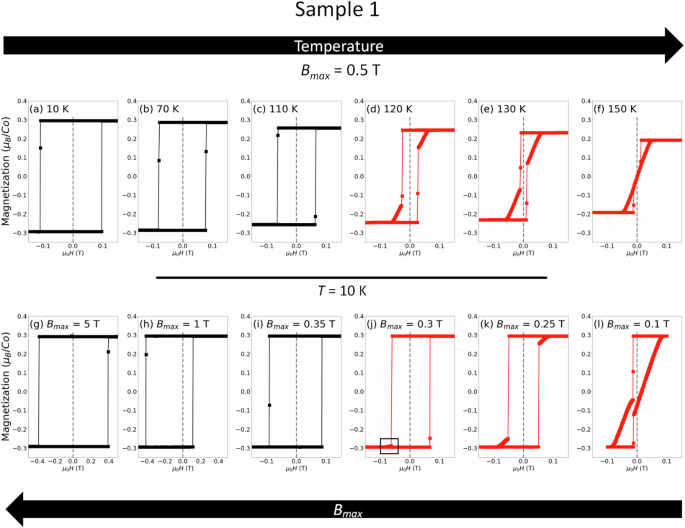
a–f Hysteresis loops at 10 K, 70 K,110 K, 120 K, 130 K, 150 K, all with an identical maximum sweeping magnetic field (B_max = 0.5 T). Note the emergence of a bow-tie feature above 120 K. g–l Hysteresis loops at T = 10 K with different maximums sweeping fields (B_max = 5 T, 1 T, 0.35 T, 0.3 T, 0.25 T and 0.1 T). When B_max becomes smaller than 0.35 T, a bow-tie feature emerges.

Full size image

The evolution seen in Fig. 2a–f is similar to what was reported by Lachman et al.²¹, who found that the hysteresis loop acquires a ‘bow-tie’ shape above a threshold temperature. The only difference is that our threshold temperature (T_A = 115 K ± 5 K) is lower than theirs (T_G = 125 K). This difference will be explained at the end of this paper. Another feature which appears at low temperature is a genuine asymmetry between positive and negative orientations : B₀₊ ≠ B₀₋²¹, which is particularly visible in Fig. 2h.

Panels g-l in figure 2 show the hysteresis loops at 10 K with different maximum sweeping fields, B_max. The evolution is similar to the one induced by warming. When B_max = 5 T, the magnetization loop is rectangular. Decreasing B_max reduces B₀, in agreement with what was previously reported²⁴. For sufficiently small B_max (that is, when B_max < 0.35 T), the hysteresis loop acquires a bow-tie shape. The emergence of bow-tie shape and low values of B₀ are concomitant. We refer to the amplitude of B₀ below which the hysteresis loop displays a bow-tie feature as ({B}_{0}^{bt}).

Thus, at low temperature, the shape of the hysteresis loop and the amplitude of B₀ both depend on B_max. In other words, the amplitude of magnetization at a given magnetic field does not exclusively depend on temperature and magnetic field, but also on the magnetic field applied in the past. If the latter is not large enough, a memory persists. Memory formation in condensed matter is defined as an ‘ability to encode, access, and erase signatures of past history in the state of a system’²⁹. The present case is reminiscent of another topological magnet, namely Mn₃X (either with X=Sn³⁰ or X=Ge³¹). However, as we will see below, here the information is stocked not in the domain walls between antiferromagnetic domains, but in a secondary spin population.

Origin of the Bow-tie shape

Multiplicity of magnetic domains in Co₃Sn₂S₂, which occurs when the amplitude of magnetization is below its peak value of M_s ≃ 0.3 μ_B/Co, has been probed by microscopic techniques^17,32,33. To identify the origin of ({B}_{0}^{bt}) and the change in the shape of the hysteresis loop across this threshold, we scrutinized hysteresis loops with a very small (< 0.2 T) B_max, leading to a magnetization lower than M_s.

Figure 3a illustrates the variation of magnetization with applied magnetic field during three successive hysteresis loops where the amplitude of B_max is incrementally reduced after each loop. The first two loops (blue and green) have a bow-tie shape: magnetization is first flat, then abruptly drops (or jumps) and then shows a steady drift towards its saturated value with a slope tending to be independent of B_max. During this steady drift, the system hosts multiple magnetic domains. In the third loop (red), B_max is so low that abrupt jumps (or drops) vanish. Note that the slope of magnetization in the red loop is similar to the slope of magnetization in the green and blue loops which presents a bow-tie shape. This slope, which does not depend on B_max, sets ({B}_{0}^{bt}). Dividing μ₀M_s by dM/dH yields 85 mT (Fig. 3a), close to the threshold ({B}_{0}^{bt}) revealed in the transition between panels i and j of Fig. 2.

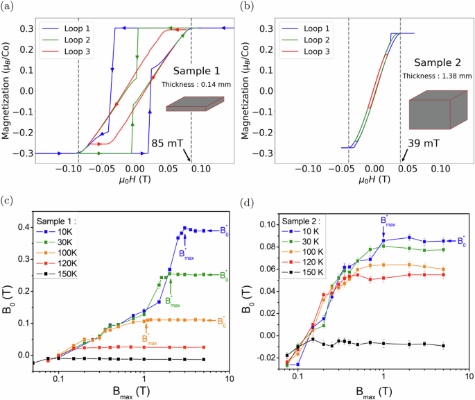
a Three Magnetization loops at 10 K. Loop 1 (blue): starting field at 0.2 T. Loop 2 (green): starting field at 0.1 T. Loop 3 (red): starting field at 0.08 T. b Loops for a thicker sample. Loop 1 (blue): starting field at 0.06 T. Loop 2 (green): starting field at 0.04 T. Loop 3 (red): starting field at 0.02 T. Bow-tie features tend to two parallel lines. c B₀ as function of B_max at different temperatures for sample 1; d Same for sample 2. At each temperature, B₀ initially increases linearly with increasing B_max. It eventually saturates to a constant value. This threshold sweeping field, ({B}_{rm{max}}^{star }), is shown by arrows. The saturated amplitude of B₀, called ({B}_{0}^{star }) is also shown. Both ({B}_{0}^{star }) and ({B}_{rm{max}}^{star }) decrease with increasing temperature.

Full size image

Magnetization loops for a thicker sample (Fig. 3b) are similar, but there is a quantitative difference. The magnetization slope is steeper in the thicker sample, which has almost a cubic shape. M_s is identical in the two samples and therefore the threshold field is reduced to 39 mT in this thicker sample. Thus, with increasing thickness, the multi-domain window becomes narrower, the magnetization slope becomes steeper and ({B}_{0}^{bt}) is reduced.

The difference in the demagnetizing factors of the two samples provides a quantitative account of this thickness dependence. As seen in Table 1, D, the demagnetizing factor calculated by using the formula for a rectangular prism³⁴, is very close to (frac{dH}{dM}), the inverse of the magnetization slope measured in the experiment.

When the magnetic field becomes equal to B_0±, an energy barrier is crossed and spins flip to the opposite orientation. If ∣B_0±∣ ⩾ μ₀DM_s, the spin-flip is total and the loop is rectangular. On the other hand, if ∣B_0±∣ ⩽ μ₀DM_s, spin-flip is partial and the loop has a bow-tie shape, because a multi-domain configuration is stable thanks to the demagnetization energy. This leads us to ({B}_{0}^{bt}={mu }_{0}D{M}_{s}), in agreement with the experimental observation.

Temperature dependence of the memory effect

We saw that the magnitude of B₀ depends on the maximum sweeping field, B_max. Figure 3c illustrates this dependence for different temperatures in a semi-log plot. At each temperature, the initial increase B₀, which is roughly linear in B_max ends by saturation to a constant value, which we dub ({B}_{0}^{star }). Let us call ({{rm{B}}}_{rm{max}}^{star }) the magnitude of B_max above which ({B}_{0}={B}_{0}^{star }). As one can see in the figure, both ({B}_{0}^{star }) and ({B}_{rm{max}}^{star }) steadily decrease with increasing temperature. The picture drawn by this data is following: when ({B}_{rm{max}} ,<, {B}_{rm{max}}^{star }), the system has a memory, which shows itself in the magnitude of B₀. Spin flip occurs at a threshold magnetic field, which depends on the previously visited field. When ({B}_{rm{max}},>,{B}_{rm{max}}^{star }), there is no such memory and ({B}_{0}(T)={B}_{0}^{star }(T)) is independent of previous history.

Figure 3d presents the same data for the thicker sample (#2). The behavior is qualitatively similar: After an initial increase, B₀ saturates at a temperature dependent magnitude. Note, however, that the absolute value of ({B}_{0}^{star }) is much smaller in the thicker sample. At low temperature, ({B}_{0}^{star }simeq 0.4) T in sample 1 and ({B}_{0}^{star }simeq 0.09) T in sample 2. It is noteworthy that, for both samples, ({B}_{rm{max}}^{star }/{B}_{0}^{star }approx 8) and this ratio does not show any strong temperature dependence. This indicates that the temperature-induced decrease in both field scales is similar.

({B}_{0}^{star }) is the coercive field of the system when the memory is erased. As expected³⁵, it decreases with increasing temperature. Its amplitude in the zero-temperature limit is much smaller than the magneto-crystalline anisotropy field, i.e. to the in-plane magnetic field needed to saturate magnetization. The latter is as large as ~23 T³⁶. This difference makes Co₃Sn₂S₂ another example of what is known as ‘Brown’s coercivity paradox’³⁷. Experiments have found that the coercivity is often much smaller than the lowest bound expected according to the magneto-crystalline anisotropy³⁸. It has been shown that large demagnetizing fields developed near sharp corners play a significant role in setting coercivity³⁷ and imperfections can reduce the expected coercive field³⁹.

Thus, when the maximum sweeping field B_max becomes lower than a threshold (({B}_{rm{max}}^{star })), B₀ becomes lower than its peak value ({B}_{0}^{star }simeq 0.4) T. Moreover, this is also the case of the difference between ∣B₀₊∣ and ∣B₀₋∣, which becomes significantly larger than our experimental margin. Thus, the memory effect tunes the exchange bias, too (See the Supplementary Materials for details⁴⁰).

Zooming on saturated magnetization

Given the content of this memory, one may suspect that when it is not erased, the energy barrier between two single-domain states is attenuated. This may be caused by the presence of a secondary spin component or population which modifies the overall energy landscape and attenuates the height of the barrier. A careful examination of saturated magnetization at the end of a hysteresis loop confirms this.

Figure 4a displays three loops all at 10 K with three different endings (B_max= 0.5 T; 1.5 T and 4.8 T). The figure shows that B₀ increases with increasing B_max, as we saw above. At first sight, magnetization appears to saturate at the same amplitude. However, this is not the case. Figure 4b is a zoom on the three curves near the maximum magnetization. One can see that there is a small, yet finite difference between the three curves. With increasing B_max, the amplitude of magnetization at the end of a ‘rectangular’ loop is larger. We carefully documented the dependence of spontaneous magnetization at the end of a loop (measured at B = ± 0.05 T) on the amplitude of the sweeping magnetic field.

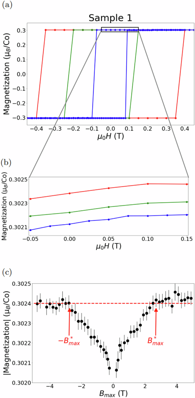
a Three magnetization loops, red : B_max = 4.8 T, green: B_max = 1.5 T and blue: B_max = 0.5 T. b Zoom in positive magnetization at low field. c B_max dependence of the absolute value of magnetization at ± 50 mT (depending on B_max sign).

Full size image

Figure 4c shows the result. The spontaneous magnetization at the end of a loop increases with increasing ∣B_max∣ before saturating to a constant value when B_max becomes equal to ({B}_{rm{max}}^{star }). The detected increase of magnetization between ({B}_{0}^{star }) (the end of the loop) and its eventual saturation above ({B}_{rm{max}}^{star }) is tiny (≈0.1%), but larger than our experimental margin. This observation has an important implication: when the sample has not visited a sufficiently large B_max, it hosts a small population of spins whose magnetization does not correspond to the polarity of majority spins. This population is where the memory is stored. The existence of a ({B}_{rm{max}}^{star }) (roughly 8 times larger than ({{rm{B}}}_{0}^{star })) is caused by this secondary spin population whose coercive field is larger and much more broadly distributed than the coercive field of the majority spins. The secondary spins, presumably three orders of magnitude more dilute than the principal population, may be situated either at the surface of the sample or at off-stoichiometric sites.

Having identified four different field scales (See Table 2), let us now turn our attention to the phase diagram.

Origin of T_A, the additional temperature scale

Figure 5a shows the evolution of ({B}_{0}^{star }) and ({B}_{0}^{bt}) with temperature. ({B}_{0}^{bt}), the threshold field for bow-tie shape, is almost flat and its absolute value coincides with μ₀DM_s. In contrast, ({B}_{0}^{star }), the saturated B₀, is temperature dependent and rapidly decreases with increasing temperature. T_A is the temperature at which ({B}_{0}^{star }) and ({B}_{0}^{bt}) cross each other. When ({B}_{0}^{star }) falls below ({B}_{0}^{bt}), whatever the sweeping field B_max, one finds ({B}_{0},<,{B}_{0}^{bt}). This makes a bow-tie shape unavoidable. Thus, no thermodynamic phase transition occurs at T_A. This temperature threshold arises as a result of the crossing between two boundaries.

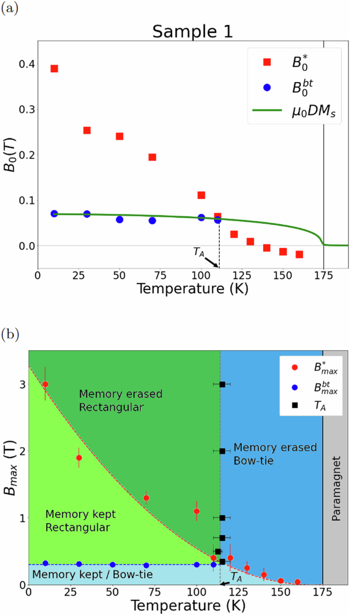
a ({B}_{0}^{star }) and ({B}_{0}^{bt}) versus temperature. The measured ({B}_{0}^{bt}) tracks μ₀DM_s (with D = 0.76), which is represented by the green solid line. ({B}_{0}^{star }) and ({B}_{0}^{bt}) cross each other at T_A. Above this, hysteresis loops can only have a bow-tie shape for whatever B_max, because of the ({{rm{B}}}_{0}^{star },<,{B}_{0}^{bt}) inequality. b ({{rm{B}}}_{rm{max}}^{star }) and ({B}_{rm{max}}^{bt}) versus temperature. Dashed lines are guides to the eye. T_A = 115 ± 5 K, corresponds to the crossing point of ({{rm{B}}}_{rm{max}}^{star }) and ({B}_{rm{max}}^{bt}).

Full size image

This is further illustrated in Fig. 5b, a representation of the evolution of ({B}_{rm{max}}^{star }) and ({B}_{rm{max}}^{bt}) in the (field, temperature) plane. When ({B}_{rm{max}},>,{B}_{rm{max}}^{star }), the system has no memory (that is, the shape of hysteresis loop does not depend on the past history) and when ({B}_{rm{max}},<,{B}_{rm{max}}^{star }), there is a memory. ({B}_{rm{max}}^{star }(T)) is the boundary between two states with and without memory. A second boundary is defined by ({B}_{rm{max}}^{bt}). When B_max is larger than this threshold, the hysteresis loop is rectangular. Since B_max/B₀ ratio does not change with temperature, T_A, the temperature at which ({B}_{rm{max}}^{bt}={B}_{rm{max}}^{star }) is similar to what can be seen in Fig. 5a. Since ({B}_{0}^{bt}) and ({B}_{rm{max}}^{bt}) depend on the demagnetizing factor and the sample morphology, the horizontal lines in these figures are expected to vary from sample to sample with the change in the aspect ratio. This would explain the fact that the reported secondary temperature differs from one study to another.

Thus, the magnetic order in Co₃Sn₂S₂ remains ferromagnetic with spins oriented along the c-axis. However, in presence of a magnetic field oriented along the c-axis, as a function of temperature and magnetic field (both at present and in the past), multiple meta-stable configurations can arise. What distinguishes them is the polarity in different sub-sets of spin population, despite the global ferromagnetic order.

Thermodynamic limit for well-defined magnetization

One manifestation of this meta-stability is the contrast between local and global magnetization, shown in Fig. 6. When the system is in the rectangular regime, local magnetization, measured with micron-sized Hall sensors (see supplementary material for details⁴⁰), is very similar to the magnetization of the whole sample. In other words, the passage between single-domain regimes of opposite polarities is almost identical everywhere in the sample (Fig. 6a, b). On the other hand, when the sample is multi-domain, while global magnetization presents a smooth and reproducible slope (Fig. 6c), local magnetization is not reproducible from one sweep to another (Fig. 6d). This confirms that when the memory is not erased, the energy landscape is not smooth⁴¹. There are numerous competing spin configurations, spatially distinct over a micrometer, but with similar global magnetization. Our case emerges as a platform for studying thermodynamics of small systems⁴².

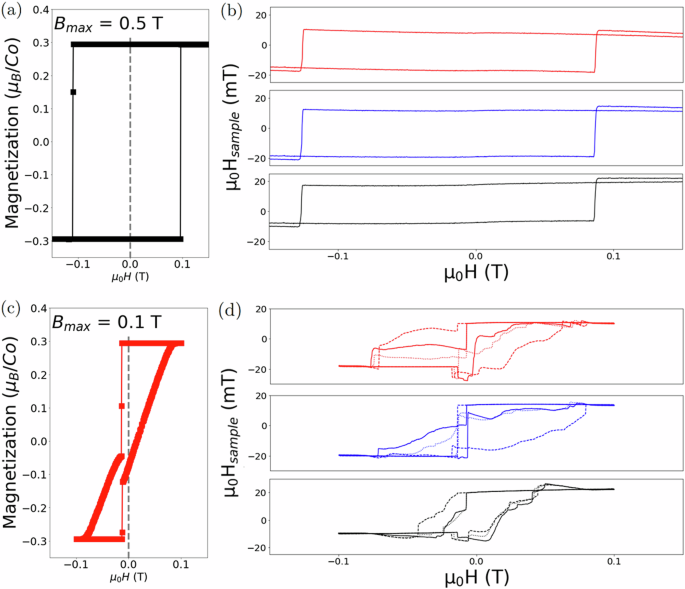
a Magnetization of the whole sample, measured with a vibrating-sample magnetometer, at 10 K for B_max = 0.5 T. b Local magnetization, measured in identical conditions by an array of 2DEG micron-sizes Hall sensors put on the surface of the sample. The three curves represent the local magnetic field at three different positions of the sample. c Magnetization of the whole sample at 10 K for B_max = 0.1 T. Hysteresis displays a bow-tie shape. d Local magnetization measured in similar conditions. Each color represents a position on the sample (three consecutive hysteresis loops were measured.).

Full size image

Possibly related phenomena in other magnetic solids

Let us note that Co₃Sn₂S₂ is not the first case of multiple spin populations. In SrRuO₃ thin films^43,44 with a thickness of few unit cells, there is an additional peak in the Hall response. It has been proposed that it is caused by contributions of opposite signs from two distinct magnetic regions with different saturation magnetizations⁴⁵. The two contributions have different coercive fields, but this difference is far below the order of magnitude difference we see in our case. A similar observation has been reported in NiCo₂O₃ thin films⁴⁶.

These observations indicate that the existence of distinct spin populations with different coercive fields in a magnet may be more common than previously thought.

In summary, we investigated the evolution of the magnetization hysteresis loop in Co₃Sn₂S₂ with temperature and with the maximum swept magnetic field, B_max. We found that, at each temperature, increasing B_max leads to an enhancement of the coercive field up to a saturation value, ({B}_{rm{max}}^{star }). In addition, the amplitude of the saturated magnetization displays a small, yet significant, dependence on B_max. This suggests the presence of a small secondary spin population with a coercive field larger than that of the main population. The memory of the last B_max is stored by this minority spins, which do not flip if the sweeping field is lower than ({B}_{rm{max}}^{star }).

A temperature scale, T_A, distinct from the Curie temperature, was identified by several previous studies. It was suggested that it corresponds to a thermodynamic phase transition within the magnetically ordered state. This secondary phase was suggested to be in-plane antiferromagnetism¹⁵, spin glass²¹ or an anomaly in domain wall mobility¹⁷. According to our study, T_A does not correspond to a thermodynamic phase transition, but to a crossing point between meta-stable states. The two boundaries which cross at T_A separate regimes with and without memory and regimes which are single-domain and multiple-domain. The origin of the two distinct coercive fields corresponding to two distinct spin populations emerges as a puzzle to be addressed by future studies.

Crystals of Co₃Sn₂S₂ were grown by self-flux method as detailed previously⁹.

Magnetization was measured using a Quantum Design MPMS in Vibrating Sample Magnetometer (VSM) mode with magnetic field applied along the crystalline c-axis with a quartz sample holder.

The hysteresis loops displayed in Figs. 2 and 3c, d, were obtained according to the following protocol :

• Set the temperature.

• Reduce the remanent field by sweeping the applied field with gradually decreasing ∣B_max∣ until finding that magnetization is not saturated anymore. For instance, the field was swept first from −0.5 T, to 0.2 T then to −0.1 T, then to 0.05 T, and finally to 0 T.

• Loops were measured consecutively, starting from the smallest to the largest B_max without additional delay between steps of measurement.

• Loops measurement were done by initially setting the external field to B_max (with a sweep rate of 100 Oe/s). Then the external field was swept at 10 Oe/s in linear mode from B_max to –B_max, then swept back to B_max.

Loops in figure 4 were obtained by decreasing B_max. They are similar to experiments performed by increasing B_max.

To measure local magnetization, we employed an array of Hall sensors based on high-mobility AlGaAs/GaAs heterostructure with a 160 nm two-dimensional electron gas (2DEG) below the surface, as done before^30,47,48. The device was fabricated using electron beam lithography and 250 V argon ions to define the mesa. The device consists of ten 5 × 5 μm² sensors separated from their neighbor by 100 μm. The hall resistance of the sensors are R_Hall ≈ 6.2 × 10³(*)B. The local magnetic field at the surface of the sample was obtained by measuring the Hall resistivity of a sensor put on the sample. The sensor resistivity was measured using a Quantum Design PPMS with applied field along the c-axis of the sample.