Mapping 1-km soybean yield across China from 2001 to 2020 based on ensemble learning

Global food security is facing challenges, particularly against the backdrop of complex political and climatic conditions¹. Among major agricultural products, soybean is not only a crucial source of protein and oil but also plays a key role in agriculture, industry, and the sustainable development of economies². High-spatial-resolution and high-accuracy soybean yield dataset is a powerful tool to provide more scientific and macroscopic perspective to investigate soybean production, thereby enhancing cultivation and management techniques effectively to ensure a stable supply of soybean. However, such kind of dataset is still limited.

Currently, the primary sources of soybean yield spatialization information include yield data recorded by agricultural meteorological stations, statistical data at administrative unit scales, and rasterized yield datasets. Despite their advantages, these datasets do have their limitations either in spatial resolution or time resolution, thus limiting their use over large areas or long time periods. For instance, the yield data recorded by agricultural meteorological stations can provide real-time, location-specific records of soybean yields, which typically possess a higher degree of accuracy³. However, such data are limited in spatial coverage making it challenging to represent the spatial variability of soybean yield over large areas. Similarly, soybean yield data at the administrative unit scales are based on statistics and records at administrative units (such as provinces, cities, and counties). These data facilitate the analysis of differences in soybean yield levels across different regions but cannot reflect spatial differences within regions^4,5. Compared with recorded data, rasterized soybean yield datasets should be able to provide high-resolution spatial data and enable a more detailed analysis of the distribution of soybean yield across different geographical locations. However, the existing commonly used rasterized soybean yield datasets such as Harvested Area and Yield for 4 Crops (EarthStat)⁶, Spatial Production Allocation Model (MapSPAM)⁷, and Global Dataset of Historical Yields (GDHY)⁸ often have low temporal or spatial resolution. The highest spatial resolution of these dataset is only 10 kilometers. Moreover, some of these datasets only contain data series for 2 or 3 years, which is not sufficient for establishing robust statistical analysis. In summary, the usability of the spatial distribution data for soybean yield is still inadequate, limiting their utility in precise agricultural planning and management. Thus, there is an urgent need to develop a dataset that features high temporal and spatial resolution, along with high precision, specifically a multi-year soybean yield spatialization dataset.

The primary approaches used to monitor crop yield are process-based crop models and statistic models^9,10. However, these two types of models are not particularly suitable for generating spatially gridded yield datasets. Process-based crop models are mathematical models based on principles of crop physiology and environmental science, but they typically require high-quality ground-based observations and extensive data inputs (such as daily-scale temperature, precipitation, and solar radiation)¹¹, making them difficult to use in data-scarce regions^12,13,14. In contrast to process-based models, statistic models link crop yield to predictor variables and calibrate empirical relationships through measurement results^15,16. Due to their simplicity of operation, statistic models are widely used for estimating crop yield¹⁷. However, these models are not without issues in the study of crop yield spatialization. Statistic models are often localized, and the empirical relationships between crop yield and predictor variables cannot be easily generalized to other regions. Moreover, traditional linear statistic models are particularly limited in capturing non-linear relationships between variables^18,19.

Machine learning models is rapidly evolving and has a wide range of applications in agricultural research²⁰. Compared to traditional process-based crop models and statistic models, machine learning models, e.g., random forest and support vector machine, can handle larger and more complex datasets, uncovering non-linear and intricate relationships within the data, thus improving the accuracy and reliability of model estimations²¹. In fact, more and more studies use machine learning models to predict crop yields^22,23,24. Additionally, machine learning models can automatically identify and leverage key features within the data and continuously improve model performance through ongoing learning and adjustments²⁵. Given its advantages in processing large datasets, it is more efficient and suitable to use machine learning models to generate rasterized crop yield maps^26,27,28,29.

Despite the above-mentioned advantages of machine learning algorithms in crop yield estimation, difference and instability were observed in their performance resulting in constrained accuracy for yield estimations³⁰. To address these issues, ensemble learning methods have recently gained prominence as a powerful technique in predictive modelling³¹. Ensemble learning involves combining the predictions of multiple models to achieve improved results over those of any single model. By aggregating diverse models, ensemble methods can reduce bias, variance, or both, and capture the underlying data distribution better, thereby yielding more accurate estimation. For example, it is found that all ensemble learning models (with lower prediction bias) outperformed individual machine learning models in predicting corn yield in three US Corn Belt states³². In addition, numerous studies demonstrated the effectiveness of ensemble learning in various applications, highlighting its potential for advancing the precision of agricultural yield estimations^33,34,35. Yet, there is a lack of research on generating rasterized soybean yield maps using ensemble learning methods.

China is one of the largest soybean producers in the world. While spatialization products for wheat, rice, and corn already exist in China, such products are lacking for soybean, which is also a staple food crop. Therefore, this study aims to use ensemble learning methods and spatial decomposition techniques to generate a rasterized soybean yield map for China through the fusion of multi-source data. Specifically, our objectives are: 1) to quantify the performance of 20 machine learning models as meta-models and base models in an ensemble setting; 2) to establish the stacking models by determining the number and type of variables for base models in the ensemble; 3) to provide a rasterized soybean yield dataset for China in 2001–2020 and conduct external cross-validation to verify its accuracy.

Study area

Influencing factors on soybean cultivation showed large variation across different regions in China due to its vast territory. Our study divided China into 3 major soybean production regions, which were furtherly divided into 10 sub-regions³⁶, as shown in Fig. 1. The 3 main production regions were the Northern Production Region (NPR), the Huang-Huai-Hai Production Region (HPR), and the Southern Production Region (SPR) (Fig. 1 and Table 1). These sub-regions were treated as dummy variables and included in the machine learning models in the subsequent analysis. Dummy variables are commonly used in regression analysis to represent categorical variables that have more than two levels. In addition, the soybean planting raster (Fig. 1) was extracted from Tibetan Plateau Data Center (TPDC)³⁷, and details of this dataset can be found in Adalibieke W et al.’s study³⁸.

Spatial distribution of 3 major soybean production regions and 10 sub-regions in China. NPR is the Northern Production Region; HPR is the Huang-Huai-Hai Production Region; SPR is the Southern Production Region.

Full size image

Data collection

Data used in this study (Table 2), mainly includes: (1) Yield data: municipal- and county-scale soybean yield data, yield data recorded by agricultural meteorological stations, and three commonly used rasterized soybean yield datasets; (2) Environmental data: climate data, remote sensing data, management data, and soil data. Detailed information at the dataset level is described in the subsequent sections.

Soybean yield data

The soybean yield data at the municipal and county scales from 2001 to 2020 were all obtained from the statistical yearbooks of the cities and counties in China. These statistical yearbooks are readily available through searching the names of the cities or counties on the China Economic and Social Big Data Research Platform (https://data.cnki.net/). Unreasonable soybean yield data including those from regions with minimal soybean cultivation areas or those affected by administrative boundary adjustments were excluded during data compilation and statistical analysis. Moreover, data on soybean production from Hong Kong, Macau, Taiwan, and islands were not available. For other regions where direct yield data were not provided, it was calculated by dividing total soybean production by planting area. All yield data was standardized to units of t/ha. In total, the collected valid data comprised 3632 entries at the municipal scale and 13854 entries at the county scale. The soybean yield data recorded by agricultural meteorological stations was extracted from the National Meteorological Science Data Center (https://data.cma.cn/article/getLeft/id/251/keyIndex/6.html) upon reasonable request. Finally, we adopted all municipal-scale recorded yield data (2001–2020) to establish the model and generate the dataset. Then, we comprehensively validated our dataset and the commonly utilized rasterized soybean yield datasets (EarthStat⁶, MapSPAM⁷, and GDHY⁸) using both station- and county-scale recorded yield data to enhance the reliability of our results. It should be noted that we have previously used county-scale recorded yield data to establish the model and municipal-scale data for model validation and accuracy assessment. However, the model’s performance was not as good as the results obtained using the current method.

Climate data

The most commonly used climate factors include temperature, precipitation, and solar radiation. These factors have impact on different stages of soybean growth and nitrogen-related processes, thereby affecting soybean yield^39,40. In addition, drought occurs frequently in China with averaged frequency about every 2.7 years, which can significantly impact soybean yield⁴¹. PDSI assesses agricultural drought conditions by considering factors such as precipitation, soil moisture, and vegetation growth⁴². VPD is another factor have influence on stomatal conductance and photosynthesis, thus influencing soybean growth^43,44. Therefore, in addition to commonly used climate factors, this study also incorporated PDSI and VPD as predictor variables to enhance the accuracy of soybean yield estimation.

Precipitation data were sourced from NOAA’s PERSIANN-CDR dataset^45,46. PERSIANN-CDR was created using an artificial neural network to estimate precipitation from remote sensing information, combined with bias correction using data from the Global Precipitation Climatology Project (GPCP). This dataset has a spatial resolution of 0.25° and a temporal resolution of 1 day. Other key climate data, including temperature, PDSI, SRAD, and VPD, were obtained from TerraClimate⁴⁷. TerraClimate is a global climate dataset that integrates satellite observations, ground-based observations, and climate model simulation results. These data have a monthly temporal resolution and an approximate spatial resolution of 4 km. In addition, we did not use the precipitation data from TerraClimate because we intended to avoid potential correlations between different variables from the same data source. Such correlations might arise from similar data processing methods used within a single dataset.

Remote sensing data

Remote sensing data provide real-time monitoring and extensive spatial coverage, offering precise information on crop growth conditions and productivity. This technology has been widely employed in estimating soybean yield^48,49,50. SIF (solar-induced chlorophyll fluorescence) from the GOSIF dataset shows a strong linear relationship with NPP at the ecosystem scale, significantly influencing soybean photosynthesis^51,52,53. NDVI is frequently used as a variable in crop yield estimation due to its ability to assess vegetation cover, growth status, and health^26,54,55. Numerous studies have utilized NDVI as a variable for monitoring soybean yield^56,57. Compared to meteorological data and other factors influencing crop growth, remote sensing data can directly reflect and monitor crop growth conditions in real-time, demonstrating substantial potential for soybean yield estimation¹⁶.

SIF data were obtained from the GOSIF dataset⁵¹, covering the period from 2001 to 2020. GOSIF has a temporal resolution of 8 days and a spatial resolution of 1 km. This dataset is a global rasterized SIF dataset generated using machine learning models from SIF observations of the Orbiting Carbon Observatory-2 (OCO-2). Additionally, this study utilized three remote sensing data products: NPP, NDVI, and LSTd, sourced from the MOD17A3HGF⁵⁸, MOD13A3⁵⁹, and MOD11A2⁶⁰ datasets, respectively. MODIS satellite remote sensing datasets provide global coverage with medium spatial and temporal resolution, offering various remote sensing products⁶¹.

Management data

The application of nitrogen fertilizer involves complex interactions with factors such as root activity and photosynthesis, which are crucial for crop yield⁶². Appropriate use of nitrogen fertilizer can enhance soybean yield⁶³. Therefore, incorporating nitrogen fertilizer application as a predictor variable for soybean yield can contribute to more accurate yield mapping. The data on soybean harvested areas and the application of fertilizers such as AS, MA, NPK, Urea, and ONS were obtained from the global crop-specific nitrogen fertilizer dataset³⁸ hosted on TPDC. This dataset includes annual data on soybean planting areas and fertilizer usage from 2001 to 2020, with a spatial resolution of 10 km. Additionally, soybean growth period data at the station scale can be obtained from the Dataset of Growth and Development of Major Crops in China (https://data.cma.cn/article/getLeft/id/251/keyIndex/6.html) upon reasonable request.

Soil data

The soil in different regions of China varies significantly, e.g., black soil in the northeast and red soil in southern China. Different soil types are suitable for cultivating different soybean varieties⁶⁴ and soybean yield and quality are influenced by different soil characters. For instance, Anthony et al. found a negative correlation between soybean yield and soil pH across all locations and years⁶⁵; Ferreira et al. confirmed that certain soil physicochemical properties, such as REF_BULK, OC, and SM, affect soybean yield⁶⁶. Therefore, this study incorporated all these soil variables as predictors to improve the accuracy of soybean yield estimation.

The soil physicochemical properties data except SM were sourced from the Harmonized World Soil Database (HWSD) version 2.0, which compiles soil information from around the globe into a standardized, globally consistent soil dataset. HWSD provides soil data at a 1-km resolution from 2007⁶⁷. As to SM data, they were obtained from TerraClimate⁴⁷, which estimates soil water content by integrating climate inputs with a hydrological model. We used soil data for a depth of 1 meter, as the root systems of soybeans are generally confined to this depth range. Additionally, soil data may be provided in multiple layers. If so, we would weight-average the data according to the thickness of each soil layer.

Modelling methods

Figure 2 delineates the entire process of estimating soybean yield in China based on a stacking model. Initially, the collected data on soybean, climate, remote sensing, management, and soil were preprocessed through synthesized by growth stages, resampling, and masking according to growth regions. Subsequently, we evaluated the fitting performance of 20 machine learning models using climate, remote sensing, management, and soil data as predictor variables and municipal soybean yield as the response variable in each soybean production region. The five machine learning models with the best fitting performance were selected as base models. We then assessed the performance of 20 meta models in the stacking ensemble, selecting the best-performing meta model for each region. By further refining the number of base models and the combination of predictor variables, we enhanced the performance of the ensemble model. Ultimately, we established an ensemble model for estimating soybean yield in each region. The simulated rasterized soybean yield was used as a weight to spatially disaggregate the municipal-scale soybean yield, developing 1-km annual rasterized soybean yield maps for China. Finally, the results of this study, along with three commonly used datasets (EarthStat, MapSPAM, and GDHY), were then aggregated to the county-scale or extracted to the station-scale to be comprehensively validated using recorded data at county or station scales.

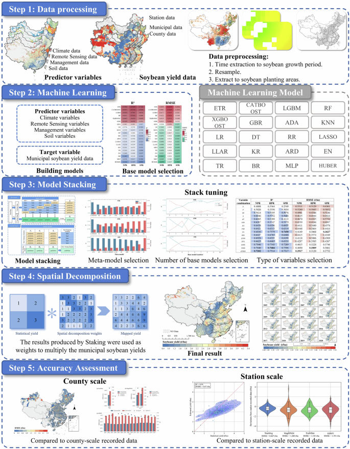
Flowchart of the proposed model stacking methodology based on multiple data sources for mapping soybean yield.

Full size image

Data preprocessing

First, we standardized the temporal scale of the data to align accurately with the soybean growth cycle by synthesizing the data based on different growth periods. By applying the kriging interpolation method to station-scale data during the soybean growth period, we generated base maps for the sowing and harvesting months. Variables with available data within the growth period were synthesized accordingly, while variables with a temporal resolution of one year or less were not processed. Next, all remote sensing images were resampled to a spatial resolution of 1-km to standardize pixel sizes and positions. Finally, using the soybean planting area as a base map, all images were masked to extract data for the soybean planting area. All data were aggregated at the municipal- and county-scale, providing the data required for model training and evaluation. The final processed predictor variables in this study can be found in Table 3.

Machine learning models

To fully leverage the capabilities of machine learning models in monitoring soybean yield, we firstly adopted a machine learning library PyCaret 3.3.1 in Python, to compare the performance of 20 machine learning models both as base models and meta models (Table 4). We tried a variety of machine learning models with the aim of screening out the better-performing ones, and the exact number of candidate models has little impact on the subsequent analysis. To ensure a fair comparison, all models were used with their default parameters (Table 5). Results showed that ETR and CATBOOST consistently exhibited outstanding performance across different regions (Fig. 5). In addition, XGBOOST, LGBM, and RF also showed excellent performance. In summary, ETR, CATBOOST, XGBOOST, LGBM, and RF were used as base models. Detailed information about these 5 models was shown in the following two paragraphs, while detailed information about the other models is not provided in this study due to space limitations.

CATBOOST⁶⁸ is a machine learning model based on gradient boosting decision trees. This model can effectively handle categorical features and minimize information loss. The ETR⁶⁹ model constructs multiple decision trees and combines their results to produce final predictions. Unlike other models, ETR uses the entire training sample at each split point rather than a random sample, and it selects split points randomly rather than optimally. Thus, this approach increases model diversity, reduces the risk of overfitting, and typically enhances prediction accuracy while speeding up the tree-building process due to its randomness.

XGBOOST⁷⁰ is an efficient gradient boosting decision tree (GBDT) algorithm that employs various optimization techniques including approximate greedy algorithms, distributed computing, and caching to accelerate the training process. Consequently, XGBOOST has its advantage in superior accuracy and speed. LGBM⁷¹ is another GBDT algorithm that uses a histogram-based decision tree algorithm to discretize continuous features, significantly reducing memory consumption and computation time. RF⁷² is a popular machine learning model widely used for crop yield prediction. It generates prediction results by multiple decision trees and aggregates them through voting or averaging. Compared to a single decision tree, RF reduces overfitting and is more robust in handling high-dimensional and missing data.

Model stacking

Stacking is an ensemble learning algorithm that utilizes the output variables of multiple base models as feature variables to train a meta-model, which predicts the final target variable⁷³. In stacking, the performance of the ensemble model can be enhanced by selecting the base models and meta-model with the best evaluation results. To our knowledge, this algorithm has rarely been applied in studies on yield spatialization. Figure 3 illustrates the principle of the stacking model. In this study, a 5-fold cross-validation method was used to combine base models.

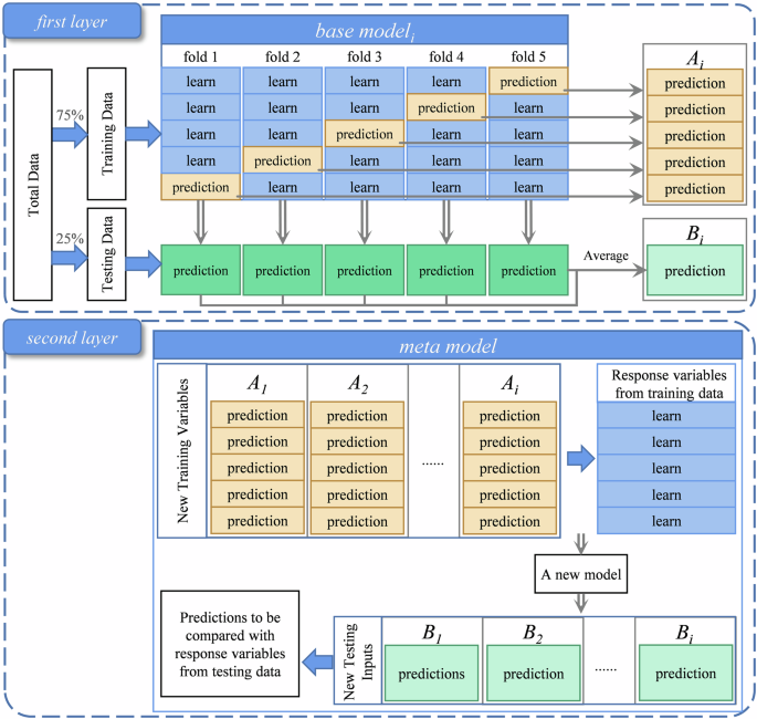
Schematic representation of the proposed 5-fold cross-validation based stacking model approach.

Full size image

In the first layer, during the execution of each base model, 75% of the data is used as the training set, and 25% as the test set. The training set is then randomly divided into five parts. Each time, four parts are selected to train the model, and the remaining one part, along with the test set, is used for prediction. This process is repeated five times to obtain predictions for both the training and test sets. The predictions for the training set are stacked together to generate predictions consistent in length with the training set, while the test set predictions are averaged to produce predictions consistent in length with the test set.

In the second layer, the predictions from the i_th base models for the training set serve as input variables, and the training set serves as the response variable to train the meta-model. The test set predictions from the i_th base models are used as input variables, and the predictions of the meta-model are compared with the actual test set to evaluate the performance of the stacking model. Since the number of base models can also affect the performance of the ensemble model, this study initially employs the five best-performing base models to select the most effective meta-model. Subsequently, the precision of ensemble models composed of different numbers of base models is compared to determine the optimal number of base models for constructing the soybean yield estimation ensemble model.

Spatial decomposition

After applying ensemble learning modeling, soybean yield was estimated for each production region, resulting in rasterized soybean yield simulation maps. These maps were then used as weights to spatially disaggregate the municipal soybean yield statistics. First, the annual estimated soybean yield from 2001 to 2020 were converted into spatial disaggregation weights ({w}_{{cti}}):

where ({{rm{y}}}_{{rm{cti}}}^{{rm{pred}}}) is the predicted soybean yield for grid cell i in city c for year t, and I is the total number of grid cells within the city. Next, the municipal-scale statistical soybean yield data ({Y}_{{ct}}^{{stat}}) for city c were disaggregated to the grid scale, generating the spatially disaggregated soybean yield for each grid cell ({y}_{{cti}}):

Accuracy assessment

The results of this study, ChinaSoyYield1km⁷⁴, along with three commonly used datasets (EarthStat, MapSPAM, and GDHY), were then aggregated to the county-scale or extracted to the station-scale to be comprehensively validated using recorded data at county or station scales. Specifically, we calculated the coefficient of determination (R²) and root mean square error (RMSE) between the recorded data and four datasets: EarthStat, MapSPAM, GDHY, and ChinaSoyYield1km. Both EarthStat and MapSPAM have a spatial resolution of 10 km but only provide data for specific years. In contrast, GDHY contains data from 2001 to 2016, but with a spatial resolution of only 55 km. Therefore, this study enhances the credibility of accuracy assessment by conducting a comprehensive comparison with these three commonly used datasets. The coefficient of determination (R²) and root mean square error (RMSE) were given by the following equations:

where n is the number of samples, O_i and P_i denote statistical and estimated soybean yield, respectively; correspondingly, (bar{O}) and (bar{P}) represents the mean of statistical and estimated soybean yield. Generally, model’s performance become more accurate as RMSE approaching to 0 and R² approaching to 1.

Model fitting

Correlation analysis of all variables

Correlation analysis clearly illustrates whether there are significant relationships between each predictor variable and the target variable. Figure 4 shows the correlation between soybean yield and each predictor variable for each production region. Among all variables, climate variables show the strongest correlation with soybean yield. Specifically, Tmax and Tmin exhibit a strong positive correlation with soybean yield in all three regions, indicating that soybean growth is highly sensitive to temperature.

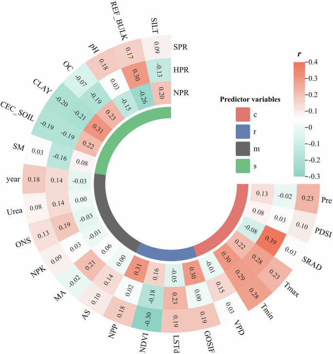
The Pearson correlation between soybean yield and predictor variables in different production regions. Note: c: climate variables; r: remote sensing variables; m: management variables; s: soil variables.

Full size image

Among the remote sensing variables, GOSIF and NPP display a strong positive correlation with soybean yield in NPR, while LSTd shows a strong positive correlation with soybean yield in HPR. In SPR, due to the warm and humid climate, the vegetation index is generally higher. However, soybean, compared to tall crops like corn or certain grains, have smaller leaf areas and thus lower vegetation indices, resulting in a strong negative correlation between NDVI and soybean yield. In comparison to other variables, management variables show a weaker correlation with soybean yield but exhibit distinct characteristics.

All management variables have a negative correlation with soybean yield in NPR, while they show a positive correlation in both HPR and SPR. The correlations of soil variables with soybean yield vary significantly across different regions. CEC_SOIL, CLAY, and OC exhibit a strong positive correlation with soybean yield in NPR but a negative correlation in HPR and SPR. Conversely, REF_BULK and pH show a strong negative correlation with soybean yield in NPR and a strong positive correlation in HPR and SPR.

In summary, these variables show a significant correlation with soybean yield across three production regions. Therefore, they can be utilized as predictor variables in subsequent soybean yield forecasting models. In addition, we did not consider the correlations among the predictor variables or the potential issue of multicollinearity. This is because we prioritize model accuracy over the interpretability of variable impacts, so we prefer to retain more information in our subsequent model construction.

Performance evaluation of individual models

We ran 20 machine learning models separately in the three soybean production regions, evaluating their performance by comparing R² and RMSE, as shown in Fig. 5. The five best-performing models were ETR, CATBOOST, LGBM, RF, and XGBOOST. These models achieved R² values above 0.64 and RMSE values below 0.44 t/ha in all regions. Consequently, these five models were selected as the base models for subsequent meta-model selection.

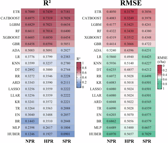
The average of model performance measurements (R² and RMSE) with 20 machine learning models.

Full size image

Selection of meta-model in stacking

Meta-model plays a crucial role in stacking models by reducing bias among individual models and enhancing the generalization ability of the ensemble. We used the five best-performing models as base models and trained 20 meta-models separately in the three production regions. Figure 6 displays the top 10 meta-models with the best simulation performance for each soybean production region. Compared to individual base models, the stacking ensemble model achieved improved modeling accuracy in each soybean production region. CATBOOST performed the best as a meta-model in NPR, with R² improving to a maximum of 0.72 and RMSE decreasing to a minimum of 0.39 t/ha. Similarly, in HPR, CATBOOST also exhibited the best performance, with R² improving to a maximum of 0.75 and RMSE decreasing to a minimum of 0.31 t/ha. In SPR, however, ETR demonstrated the best performance as a meta-model, with R² improving to a maximum of 0.73 and RMSE decreasing to a minimum of 0.38 t/ha. Therefore, we selected CATBOOST as the meta-model for constructing ensemble models in NPR and HPR, and ETR as the meta-model in SPR.

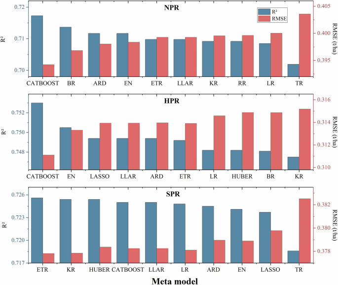
The top 10 meta-models with the best performance in terms of R² and RMSE in different soybean production regions.

Full size image

Selection of the number of base models

The results of the base models serve as the variables for the meta-model. Therefore, the number of base models can significantly impact the performance of the ensemble model. We used the meta-models to select the optimal number of base models for ensemble model performance in each of the three production regions. Figure 7 illustrates the performance of the meta-model when selecting the top 2 to top 10 base models for each soybean production region, showing different trends across regions. In comparison to fixing the number of base models at 5, in NPR, increasing the number of base models to 7 resulted in the meta-model achieving the highest performance improvement, with R² increasing from 0.7173 to 0.7197 and RMSE decreasing from 0.3942 to 0.3928. In HPR, the best performance of the meta-model was achieved with 5 base models. In SPR, the optimal performance of the meta-model was observed with 2 base models, where R² improved from 0.7256 to 0.7320 and RMSE decreased from 0.3778 to 0.3732. Therefore, in this study, we selected the top 7, 5, and 2 models based on their performance as base models for NPR, HPR, and SPR, respectively.

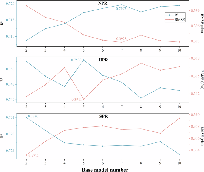
The R² and RMSE of the ensemble model when selecting 2 to 10 base models.

Full size image

Predictor variables selection

Different combinations of predictor variables can affect the performance of machine learning models. While multidimensional variables may enhance performance, they can also lead to overfitting. We evaluated the performance of the meta-model across 15 different combinations of variables in Fig. 8, based on the optimal meta-models and base models. In NPR, the meta-model achieves optimal performance when all four predictive variables are inputted. In HPR, the meta-model’s performance peaks when the input variable is rms, with R² improving from 0.7514 to 0.7684 and RMSE decreasing from 0.3120 to 0.3009. Similarly, in SPR, further performance enhancement is observed when the input variable is rs, with R² increasing from 0.7317 to 0.7458 and RMSE decreasing from 0.3732 to 0.3627. Therefore, in this study, we selected crsm, rms, and rs as the input variables for the ensemble model in NPR, HPR, and SPR, respectively. Finally, by selecting meta-models, base models, and input variables, we constructed soybean yield estimation ensemble models separately for the three production regions. Details are presented in Table 6.

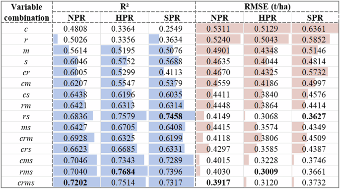
The ensemble learning fitting performance of different variable combinations in different soybean production regions. Note: c: climate variables; r: remote sensing variables; m: management variables; s: soil variables; cr: climate and remote sensing variables; cm: climate and management variables; cs: climate and soil variables; rm: remote sensing and management variables; rs: remote sensing and soil variables; ms: management and soil variables; crm: climate, remote sensing and management variables; crs: climate, remote sensing and soil variables; cms: climate, management and soil variables; rms: remote sensing, management and soil variables; crms: climate, remote sensing, management and soil variables.

Full size image

The derived yield dataset for ChinaSoyYield1km⁷⁴ during 2001–2020 is available at https://doi.org/10.57760/sciencedb.18390. The dataset is stored in GeoTiff format under the EPSG: 4326 (GCS_WGS_1984) spatial reference, with the unit of kg/ha. We did not use the unit of kg/ha as presented in this study because using the unit of kg/ha can reduce the data file size by half, making it more convenient for users to download and store. The maps can be visualized and analyzed using software such as ArcGIS, QGIS, or similar applications (Fig. 9).

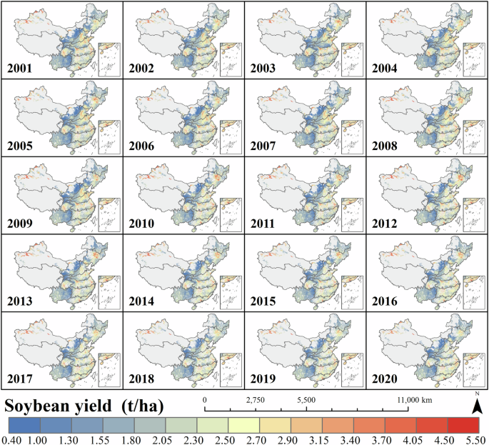
Visualization of the ChinaSoyYield1km dataset.

Full size image

We compared four datasets, including the ChinaSoyYield1km, EarthStat, MapSPAM, and GDHY, with recorded yield data at both county and station scales (data not used in our model development process). Overall, both at the county and station scales, the soybean yield estimates in this study demonstrate higher accuracy compared to the three commonly used datasets.

We first aggregated the 2001–2020 ChinaSoyYield1km estimates and the EarthStat, MapSPAM, and GDHY rasterized yield estimates to the county scale and compared them with recorded data. Figure 10 shows the root mean square error (RMSE) between the ChinaSoyYield1km and recorded soybean yield. At the county scale, the RMSE between the results of this study and the recorded data is generally within the range of 3.90 t/ha. In over 90% of the regions, the RMSE for soybean yield is within 2.10 t/ha, with only a few counties having RMSE outside the reasonable range, indicating the high accuracy of the soybean yield data generated in this study.

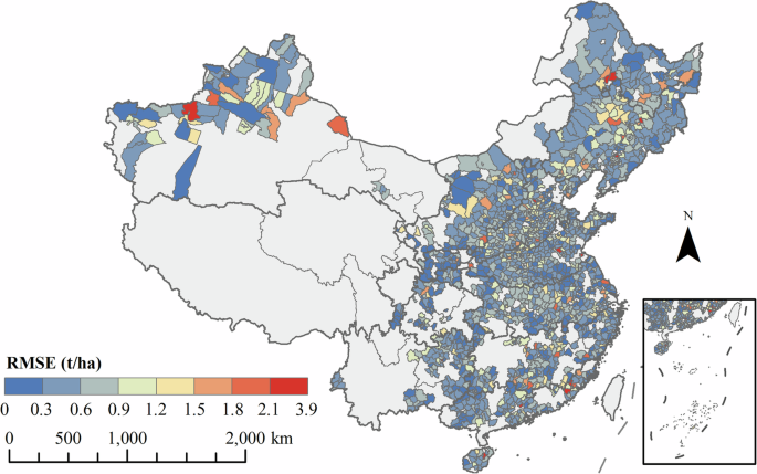
The RMSE between the results of our stacking model and recorded data at the county scale.

Full size image

Figure 11 presents the R² and RMSE for four datasets, each compared to the recorded data. Due to the temporal resolution limitations of the EarthStat and MapSPAM data, comparisons could only be made for specific years. It can be seen that in 2005 and 2010 (Fig. 11a and b), the R² values for our dataset were over 0.50, and when compared to GDHY (Fig. 11c), they were also above 0.50 in most years. This indicates that our resulting dataset captures over 50% of the yield variability at the county scale, demonstrating superior accuracy compared to publicly available datasets. The RMSE results also illustrate the same fact. The RMSE of our dataset compared to the county-scale recorded data was lower than that of existing datasets in all years, with reductions ranging from 0.18 to 0.60 t/ha.

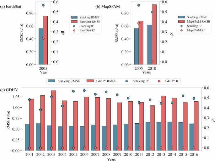
The RMSE and R² between the recorded data at the county scale and the results of our stacking model as well as three existing rasterized yield datasets (EarthStat, MapSPAM, and GDHY).

Full size image

We extracted the station-specific yield estimates from the ChinaSoyYield1km dataset, as well as from the EarthStat, MapSPAM, and GDHY datasets, and compared them with station-recorded data. Figure 12 shows that the R² between the results of this study and the station-recorded data is 0.30, with an RMSE of 0.67 t/ha. The station-recorded data mainly range between 1.50–3.00 t/ha, within which the soybean yield estimates from this study show high consistency with the station-recorded data. Figure 13 compares the RMSE of the deviations between the estimated yield from the four datasets and the station-recorded yield. The data from this study show the smallest deviations, all within 2.00 t/ha, whereas the deviations for MapSPAM and GDHY exceed 3.00 t/ha. The average and peak deviations of the data from this study are closest to 0 t/ha when compared to station-recorded yield. Although EarthStat shows fewer extreme values, its average deviation from station-recorded yield is the largest. Due to its lower spatial resolution, GDHY shows relatively lower accuracy at the station scale and contains numerous extreme values. The RMSE between the results of this study and the station-recorded yield is 0.67 t/ha, which is smaller than the RMSE of other raster yield datasets when compared to station-recorded data.

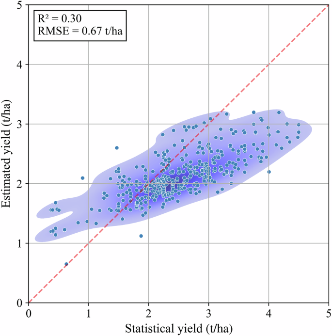
The comparison between station recorded soybean yield and the results of our stacking model.

Full size image

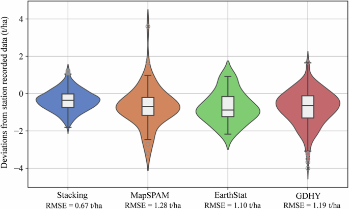
The comparison between station recorded soybean yield and the results of our stacking model as well three existing rasterized yield datasets.

Full size image

Advantages of ChinaSoyYield1km

This study has generated a 1-km rasterized soybean yield dataset for China. To our knowledge, previous research has produced distribution maps of major soybean production areas in China, but these maps were at lower spatial resolutions. High-resolution yield datasets offer more precise spatial information on crop production, enabling rapid monitoring and analysis of large agricultural regions. This, in turn, facilitates the timely implementation of appropriate measures to enhance agricultural productivity.

This study has generated an annual soybean yield dataset for China spanning the period from 2001 to 2020. Understanding the long-term trends in soybean production over the past two decades is highly significant. Analyzing these temporal dynamics can assist agricultural decision-makers, researchers, and policymakers in comprehending the changing patterns of soybean yield. This understanding can inform the development of agricultural policies, resource allocation strategies, and management practices aimed at enhancing the efficiency and stability of soybean production. Ultimately, these efforts contribute to better meeting food demand.

Limitations of ChinaSoyYield1km

The data used in this study, including remote sensing, climate, management, and soil data, are subject to uncertainties. During data preprocessing, all data were resampled to a 1-km resolution. Additionally, not all areas within each 1 km × 1 km grid may be planted with soybeans; in some cases, only a small portion of the land within the grid may be cultivated with soybeans. These issues may lead to some loss of surface information and introduce uncertainties in yield estimation. However, the purpose of yield spatialization is to inform potential data users about the expected yield level if soybeans are planted within a grid. Since the study is conducted at a 1-km resolution, the uncertainties arising from the aforementioned issues should be tolerable. Moreover, we believe that as higher-resolution planting area and environmental variable datasets become available in the future, such uncertainties will continue to decrease. Future research could benefit from using higher accuracy and resolution soybean planting area data, such as the 10-meter spatial resolution dataset⁷⁵, or carry out experiments to quantify the uncertainty caused by input data. This would enhance the precision of analyses and improve the reliability of yield estimations.

The uncertainty in statistical data is acknowledged in this study. The source and statistical methodologies for municipal-scale soybean yield used in modeling, as well as county-scale soybean yield used in model accuracy assessment, differ. While these data are collected and compiled by professional institutions, discrepancies in data collection methods, definitions, and classifications can introduce uncertainties in statistical data. It is important to recognize these potential sources of uncertainty when interpreting and applying statistical findings in agricultural research and policymaking.

The selection of predictor variables in this study lacks granularity. Variables were chosen based on four broad categories: remote sensing, climate, management, and soil, without considering finer subdivisions within each category. This approach may overlook the potential influence of specific sub-variables that could significantly impact soybean yield modeling. Sub-variables within these categories might not have been included in the model if their parent categories were filtered out during selection, thereby reducing the estimation accuracy of the models. Moreover, the precision of the models could also benefit from better predictor variables, such as vegetation indices like EVI (enhanced vegetation index) and GCVI (green chlorophyll vegetation index), or indices refined according to crop phenological stages. Future analyses could selectively screen individual sub-variables within each category, introduce new predictor variables, or attempt new spatialization approaches (e.g., state-of-the-art deep learning), to enhance model precision.