MARBLE: interpretable representations of neural population dynamics using geometric deep learning

Main
It is increasingly recognized that the dynamics of neural populations underpin computations in the brain and in artificial neural networks1,2,3 and that these dynamics often take place on low-dimensional smooth subspaces, called neural manifolds4,5,6,7,8,9,10,11,12. From this perspective, several works have focused on how the geometry4,7,13,14 or topology6,8,9 of neural manifolds relates to the underlying task or computation. By contrast, others have suggested that dynamical flows of neural population activity play an equally prominent role11,15,16,17 and that the geometry of the manifold is merely the result of embedding of a latent dynamical activity into neural space that changes over time or across individuals4,18. Although recent experimental techniques provide a means to simultaneously record the activity of large neuron populations19,20,21, inferring the underpinning latent dynamical processes from data and interpreting their relevance in computational tasks remains a fundamental challenge16.
Overcoming this challenge requires machine-learning frameworks that leverage the manifold structure of neural states and represent the dynamical flows over these manifolds. There is a plethora of methods for inferring the manifold structure, including linear methods such as principal-component analysis (PCA), targeted dimensionality reduction (TDR)22 or nonlinear manifold learning methods such as t-distributed stochastic neighbor embedding (t-SNE)23 or Uniform Manifold Approximation and Projection (UMAP)24. Yet, these methods do not explicitly represent time information, only implicitly to the extent discernible in the density variation in the data. While consistent neural dynamics have been demonstrated using canonical correlation analysis (CCA), which aligns neural trajectories approximated as linear subspaces across sessions and animals4,18, this is only meaningful when the trial-averaged dynamics closely approximate the single-trial dynamics. Similarly to manifold learning, topological data analysis infers invariant structures, for example, loops6 and tori9, from neural states without explicitly learning dynamics. Correspondingly, they can capture qualitative behaviors and changes (for example, bifurcations) but not quantitative changes in dynamics and geometry that can be crucial during representational drift4 or gain modulation25.
To learn time information explicitly in single trials, dynamical systems methods have been used26,27,28,29,30,31; however, time information in neural states depends on the particular embedding in neural state space (measured neurons), which typically varies across sessions and animals. The Latent Factor Analysis for Dynamical Systems (LFADS) framework partially overcomes this by aligning latent dynamical processes by linear transformations30; however, alignment is not meaningful in general as animals can employ distinct neural ‘strategies’ to solve a task32. Recently, representation learning methods such as Physics Informed Variational Auto-Encoder (pi-VAE)33 and Consistent EmBeddings of high-dimensional Recordings using Auxiliary variables (CEBRA)34 have been introduced to infer interpretable latent representations and accurate decoding of neural activity into behavior. While CEBRA can be used with time information only, finding consistent representations across animals requires supervision via behavioral data, which, like LFADS, aligns latent representations but uses nonlinear transformations. For scientific discovery, it would be desirable to circumvent using behavioral information, which can introduce unintended correspondence between experimental conditions, trials or animals, thus hindering the development of an unbiased distance metric to compare neural computations.
Here, we introduce a representation learning method called MARBLE (MAnifold Representation Basis LEarning), which obtains interpretable and decodable latent representations from neural dynamics and provides a well-defined similarity metric between neural population dynamics across conditions and even across different systems. MARBLE takes as input neural firing rates and user-defined labels of experimental conditions under which trials are dynamically consistent, permitting local feature extraction. Then, combining ideas from empirical dynamical modeling35, differential geometry and the statistical theory of collective systems36,37, it decomposes the dynamics into local flow fields and maps them into a common latent space using unsupervised geometric deep learning38,39,40. The user-defined labels are not class assignments, rather MARBLE infers similarities between local flow fields across multiple conditions, allowing a global latent space structure relating conditions to emerge. We show that MARBLE representations of single-neuron population recordings of the premotor cortex of macaques during a reaching task and of the hippocampus of rats during a spatial navigation task are substantially more interpretable and decodable than those obtained using current representation learning frameworks30,34. Further, MARBLE provides a robust data-driven similarity metric between dynamical systems from a limited number of trials, expressive enough to infer subtle changes in the high-dimensional dynamical flows of recurrent neural networks (RNNs) trained on cognitive tasks, which are not detected by linear subspace alignment4,13,18, and to relate these changes to task variables such as gain modulation and decision thresholds. Finally, we show that MARBLE can discover consistent latent representations across networks and animals without auxiliary signals, offering a well-defined similarity metric.
Our results suggest that differential geometric notions can reveal unaccounted-for nonlinear variations in neural data that can further our understanding of neural dynamics underpinning neural computations and behavior.
Unsupervised representation of vector fields over manifolds
To characterize neural computations during a task, for example, decision-making or arm-reaching, a typical experiment involves a set of trials under a stimulus or task condition. These trials produce a set of d-dimensional time series {x(t; c)}, representing the activity of d neurons (or dimensionally reduced variables) under condition c, which we consider to be continuous, such as firing rates. Frequently, one performs recordings under diverse conditions to discover the global latent structure of neural states or the latent variables parametrizing all tasks. For such discoveries, one requires a metric to compare dynamical flow fields across conditions or animals and reveal alterations in neural mechanisms. This is challenging as neural states often trace out complex, but sparsely sampled nonlinear flow fields. Further, across participants and sessions, neural states may be embedded differently due to different neurons recorded4,30.
To address these challenges, MARBLE takes as input an ensemble of trials {x(t; c)} per condition c and represents the local dynamical flow fields over the underlying unknown manifolds (Fig. 1a showing one manifold) in a shared latent space to reveal dynamical relationships across conditions. To exploit the manifold structure, we assume that {x(t; c)} for fixed c are dynamically consistent, that is, governed by the same but possibly time-varying inputs. This allows describing the dynamics as a vector field Fc = (f1(c), …, fn(c)) anchored to a point cloud Xc = (x1(c), …, xn(c)), where n is the number of sampled neural states (Fig. 1b). We approximate the unknown manifold by a proximity graph to Xc (Fig. 1b) and use it to define a tangent space around each neural state and a notion of smoothness (parallel transport) between nearby vectors (Supplementary Fig. 1 and equation (2)). This construction allows defining a learnable vector diffusion process (equation (3)) to denoise the flow field while preserving its fixed point structure (Fig. 1c). The manifold structure also permits decomposing the vector field into local flow fields (LFFs) defined for each neural state i as the vector field at most a distance p from i over the graph (Fig. 1d), where p can also be thought of as the order of the function that locally approximates the vector field. This lifts d-dimensional neural states to a O(dp+1)-dimensional space to encode the local dynamical context of the neural state, providing information about the short-term dynamical effect of perturbations. Note that time information is also encoded as consecutive neural states are typically adjacent over the manifold. As we will show, this richer information substantially enhances the representational capability of our method.

a, Neural activity in different trials (colors) evolving over a latent manifold. b, Vector field representation of dynamics. The nearest-neighbor graph between neural states approximates the unknown manifold. c, The vector field is optionally denoised by a trainable vector diffusion, which aligns (via parallel transport) nearby vectors while preserving the fixed point structure. d, The dynamics are decomposed into LFFs. e, LFFs are mapped one by one into latent space by a geometric deep neural network. The model infers dynamical overlaps across datasets based on similar LFFs. f, The model has three steps: feature extraction from LFFs using p-th order gradient filters; (optional) transformation into rotation-invariant features for embedding-agnostic representations (otherwise, representations are embedding-aware); and mapping features into latent space using a multilayer perceptron. g, Using the continuity over the manifold, the network is trained using unsupervised contrastive learning, mapping neighboring LFFs close and non-neighbors (both within and across manifolds) far in latent space.
As LFFs encode local dynamical variation, they are typically shared broadly across dynamical systems. Thus, they do not assign labels to neural states as in supervised learning. Instead, we use an unsupervised geometric deep- learning architecture to map LFFs individually to E-dimensional latent vectors (Fig. 1e), which introduces parameter sharing and permits identifying overlapping LFFs across conditions and systems. The architecture consists of three components (Fig. 1f, see Methods for details): (1) p gradient filter layers that give the best p-th order approximation of the LFF around i (Supplementary Figs. 1–3 and equation (8)); (2) inner product features with learnable linear transformations that make the latent vectors invariant of different embeddings of neural states manifesting as local rotations in LFFs (Extended Data Figs. 1 and 2 and equation (10)); and (3) a multilayer perceptron that outputs the latent vector zi (equation (11)). The architecture has several hyperparameters relating to training and feature extraction (Supplementary Tables 1 and 2). While most were kept at default values throughout and led to convergent training, some were varied, as summarized in Supplementary Table 3, to tune the behavior of the model. Their effect is detailed in the examples below. The network is trained unsupervised, which is possible because the continuity of LFFs over the manifold (adjacent LFFs being typically more similar (except at a fixed point) than nonadjacent ones) provides a contrastive learning objective (Fig. 1g and equation (12)).
The set of latent vectors Zc = (z1(c), …, zn(c)) represents the flow field under condition c as an empirical distribution Pc. Mapping multiple flow fields c and ({c}^{{prime} }) simultaneously, which can represent different conditions within a system or different systems altogether, allows defining a distance post hoc (d({P}_{c},{P}_{{c}^{{prime} }})) between their latent representations ({P}_{c},{P}_{{c}^{{prime} }}), reflecting the dynamical overlap between them. We use the optimal transport distance (equation (13)) because it leverages information of the metric structure in latent space and generally outperforms entropic measures (for example, Kullback–Leibler (KL) divergence) when detecting complex interactions based on overlapping distributions37.
Embedding-aware and embedding-agnostic representations
The inner product features (Fig. 1f) allow two operation modes. As an example, consider linear and rotational flow fields over a two-dimensional (2D) plane (d = 2, trivial manifold) in Fig. 2a. As shown later, MARBLE can also capture complex nonlinear dynamics and manifolds. We have labeled these flow fields as different conditions (treating them as different manifolds) and used MARBLE to discover a set of latent vectors that generate them.
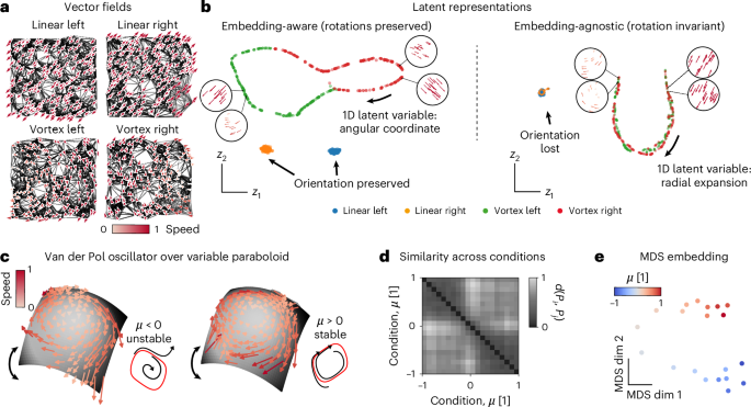
a, Four toy vector fields sampled uniformly at random over a flat (trivial) manifold approximated by a graph (black lines). Two constant (top) and two rotational fields (bottom). b, Embedding-aware representations distinguish rotational information in LFFs (left). The ring manifold in latent space parametrizes the angular variation (insets). Embedding-agnostic latent representations learn only vector field expansion and contraction (right). The one-dimensional (1D) manifold in latent space parametrizes the radial variation of LFFs (insets). c, Vector fields of the Van der Pol oscillator over a variable-curvature paraboloid in the unstable (μ = −0.25) and stable (μ = 0.25) regimes sampled from randomly initialized trajectories. Insets show the limit cycle in red and representative trajectories from a vertical projected view. d, Similarity across conditions based on optimal transport distance between respective MARBLE representations. Clustering indicates an abrupt dynamical change at μ = 0. e, 2D MDS embedding of the distribution distance matrix recovers the ordering of parameter μ over two weakly connected one-dimensional manifolds.
In embedding-aware mode, the inner product features are disabled (Fig. 2b, left) to learn the orientation of the LFFs, ensuring maximal expressivity and interpretability. Consequently, constant fields are mapped into two distinct clusters, whereas rotational fields are distributed over a ring manifold based on the angular orientation of LFFs (Fig. 2b, left, insets and Extended Data Figs. 1 and 2). This mode is useful when representing dynamics across conditions but within a given animal or neural network with the same neurons being sampled (Figs. 2c–e and 3a–g) or when a global geometry spanning all conditions is sought after (Fig. 4e).
In embedding-agnostic mode, the inner product features are enabled, making the learned features invariant to rotational transformations of the LFFs. As a result, the latent representation of the vector field will be invariant to different embeddings (conformal maps)41, which introduce local rotations. Thus, this mode is useful when comparing systems, such as neural networks trained from different initializations (Fig. 3h–j). Our example shows that constant vector fields are no longer distinguishable based on LFF orientation (Fig. 2d, right, insets and Extended Data Figs. 1 and 2); however, we still capture expansion and contraction in LFFs over a one-dimensional manifold (Extended Data Fig. 3). In both embedding-aware and -agnostic examples, note that LFFs from different manifolds (defined by user labels) are mapped close or far away, depending on their dynamical information, corroborating that labels are used for feature extraction and not for supervision.

a, Low-rank RNN takes two stimuli as input and produces a decision variable as a read-out. b, Two representative stimulus patterns (only one stimulus is shown) and decision outcomes for the delayed-match-to-sample task. Input amplitude is controlled by the ‘gain’ during stimulus epochs (red) and is zero otherwise (gray). c, Neural dynamics of a trained rank-two RNN evolves on a randomly oriented plane. Phase portrait of field dynamics superimposed with a trajectory during a trial (orange). d, Space of input weights in a trained RNN. Colors indicate k-means clustering with two subpopulations specialized in one or the other input. Ellipses represent 3 × s.d. of fitted Gaussian distributions. e, Mean-field dynamics for gains 0, 0.32 and 1.0. f, Similarity across gain conditions (shading represents gains from 0 to 1) based on optimal transport distance between the respective embedding-aware MARBLE representations. Hierarchical clustering indicates two clusters in the nonzero gain sub-block, indicating a qualitative change point (red dashed line). g, The predicted change point corresponds to the bifurcation, causing the loss in task performance. h, Networks trained from different initializations can have different dynamics over differently embedded manifolds (solution I, II). Networks sampled from the same weight distribution produce the same fixed point structure over differently embedded manifolds (solution I/1, I/2). i, Similarity across networks and gains (left) or no gain (control, middle) based on embedding-agnostic representations. We compare this to CCA (right). Shading represents gains from 0 to 1. j, MDS embedding of the distance matrices shows the continuous variation of latent states during gain modulation (left), no variation across no-gain conditions (middle) and clustering across network solutions. For CCA the same plot shows clustering across network solutions but no variation due to gain modulation.
To demonstrate embedding-agnostic mode for nonlinear dynamics on a nonlinear manifold, consider the Van der Pol oscillator mapped to a paraboloid while varying the damping parameter μ and the manifold curvature (Fig. 2c and Methods). Using short, randomly initialized simulated trajectories for 20 values of μ, labeled as different conditions, we used embedding-agnostic MARBLE to embed the corresponding vector fields into a shared latent space (E = 5). Despite the sparse sampling, we detected robust dynamical variation across conditions as μ was varied. Specifically, the similarity matrix between conditions ({D}_{c{c}^{{prime} }}=d({P}_{c},{P}_{c}^{{prime} })) displays a two-partition structure, indicating two dynamical regimes (Fig. 2d). These correspond to the stable and unstable limit cycles separated by the Hopf bifurcation at μ = 0. This result is observed independently of manifold curvature (Extended Data Fig. 4). Furthermore, and despite the sparse sampling across conditions, the two-dimensional embedding of ({D}_{c{c}^{{prime} }}) using multidimensional scaling revealed a one-dimensional manifold capturing the continuous variation of μ (Fig. 2e). Notably, manifold variation was not captured when training an embedding-aware network (Extended Data Fig. 4), confirming that embedding-agnostic representations are invariant to manifold embedding with only marginal loss of expressivity compared to the embedding-aware mode.
Comparing dynamics across recurrent neural networks
There has been a surge of recent interest in RNNs as surrogate models for neural computations15,42,43,44. Previous approaches for comparing RNN computations for a given task relied on aligning linear subspace representations of neural states14,42,45, which requires a point-by-point alignment of trials across conditions. While this is valid when the trial-averaged trajectory well approximates the single-trial dynamics4,18, it does not hold when flow fields are governed by complex fixed point structures. Thus, systematically comparing computations across RNNs requires an accurate representation of the nonlinear flow fields.
To showcase MARBLE on a complex nonlinear dynamical system, we simulated the delayed-match-to-sample task46 using RNNs with a rank-two connectivity matrix (Fig. 3a and Methods), which were previously shown to be sufficiently expressive to learn this task47. This common contextual decision-making task comprises two distinct stimuli with variable gain and two stimulus epochs of variable duration interspersed by a delay (Fig. 3b). At unit gain, we trained the RNNs to converge to output 1 if a stimulus was present during both epochs and −1 otherwise (Fig. 3b). As expected48, the neural dynamics of trained networks evolve on a randomly oriented plane (Fig. 3c). Yet we found that differently initialized networks produce two classes of solutions: in solution I the neurons specialize in sensing the two stimuli, characterized by the clustering of their input weights ({{bf{w}}}_{1}^{{mathsf{in}}},{{bf{w}}}_{2}^{{mathsf{in}}}) (Fig. 3d), whereas in solution II the neurons generalize across the two stimuli (Extended Data Fig. 5d). These two solutions exhibit qualitatively different fixed point landscapes (three fixed points for zero gain and one limit cycle for large enough gain), which cannot be aligned via continuous (linear or nonlinear) transformations (Fig. 3e and Extended Data Figs. 5c,e and 6).
We first asked whether MARBLE could infer dynamical neural correlates of loss of task performance as the stimulus gain is decreased beyond the decision threshold. For a given gain, we simulated 200 trials of different durations, sampling different portions of the nonlinear flow field due to randomness (Extended Data Fig. 6). We formed dynamically consistent datasets by subdividing trials at the stimulus onset and end to obtain four epochs. We then formed two groups, one from epochs where the stimulus was on and another where the stimulus was off (Fig. 3b). Repeating for different gains, we obtained 20 groups of stimulated epochs at different gains and 20 additional groups from unstimulated (no gain) epochs. We used the latter as negative controls because the flow fields vary across them due to sampling variability and not gain modulation. We then trained embedding-aware MARBLE to map all 40 groups, labeled as distinct conditions, into a common latent space. The resulting representational similarity matrix between conditions exhibits a block-diagonal structure (Fig. 3f). The top left block denotes distances between unstimulated controls and contains vanishing entries, demonstrating the robustness of MARBLE to sampling variability. The two bottom-right sub-blocks identified by hierarchical clustering indicate a quantitative change in dynamics, which notably corresponds to a sudden drop in task performance (Fig. 2g) from 1 to 0.5 (random). Thus, MARBLE enables the detection of dynamical events that are interpretable in terms of global decision variables.
Next, we define a similarity metric between the dynamical flows across distinct RNNs. Consider network solutions I and II, which have different flow fields (Fig. 3h) and as a negative control, two new networks whose weights are randomly sampled from the Gaussian distribution of solution I whose flow fields provably preserve the fixed point structure47. Due to the arbitrary embedding of neural states across networks, we used embedding-agnostic MARBLE to represent data from these three RNNs at different gains (E = 5). We found that latent representations were insensitive to manifold orientation, detecting similar flow fields across control networks (solutions I/1 and I/2) and different ones across solutions I and II (Fig. 3i, left). Further, the multidimensional scaling (MDS) embedding of the similarity matrix shows one-dimensional line manifolds (Fig. 3j, left) parametrizing ordered, continuous variation across gain-modulated conditions. As expected, for unstimulated conditions, we could still discriminate different network solutions but no longer found coherent dynamical changes (Fig. 3i,j, middle). For benchmarking, we used CCA, which quantifies the extent to which the linear subspace representations of data in different conditions can be linearly aligned. While CCA could distinguish solutions I and II having different fixed point structures, it could not detect dynamical variation due to gain modulation (Fig. 3i,j, right). This suggests that finding coherent latent dynamics across animals using CCA4,18 has likely succeeded in instances where linear subspace alignment is equivalent to dynamical alignment, for example, when trial-averaged dynamics well-approximate the single-trial dynamics. Here we find that MARBLE provides a robust metric between more general nonlinear flow fields possibly generated by different system architectures.
Representing and decoding neural dynamics during arm-reaches
State-of-the-art representation learning of neural dynamics uses a joint embedding of neural and behavioral signals34; however, it would be advantageous to base biological discovery on the post hoc interpretation of neural representations, which do not introduce correlations between neural states and latent representations based on behavioral signals. To demonstrate this, we reanalyzed electrophysiological recordings of a macaque performing a delayed center-out hand-reaching task30 (Methods). During the task, a trained monkey moved a handle toward seven distinct targets at radial locations from the start position. This dataset comprises simultaneous recordings of hand kinematics (Fig. 4a) and neural activity via a 24-channel probe from the premotor cortex over 44 recording sessions (Fig. 4b shows one session).

a, Ground truth hand trajectories of a macaque in seven reach conditions. Monkey image adapted by Andrea Colins Rodriguez from https://www.scidraw.io/drawing/445, CCBY 4.0. b, Single-trial spike trains in the premotor cortex for three reach conditions (24 recording channels within each color). The shaded area shows the analyzed traces after the GO cue. c, Firing rate trajectories for a reach condition (up) PCA-embedded in three dimensions for visualization. d, Vector field obtained from firing rate trajectories. e, Latent representations of neural data across conditions in a single session. CEBRA-behavior was used with reach conditions as labels. The MARBLE representation reveals as an emergent property the latent global geometric arrangement (circular and temporal order) spanning all reaches reflecting physical space. f, Linear decoding of hand trajectories from latent representations. g, Decoding accuracy measured by R2 between ground truth and decoded trajectories across all sessions for the final position (left) and instantaneous velocity (right). Two-sided Wilcoxon tests (paired samples), **P < 1 × 10⁻²; ***P < 1 × 10⁻³; ****P < 1 × 10⁻⁴; NS, not significant. Horizontal and vertical bars show mean and 1 × s.d., respectively (n = 43).
Previous supervised approaches revealed a global geometric structure of latent states spanning different reach conditions2,49. We asked whether this structure could emerge from local dynamical features in MARBLE representations. As before, we constructed dynamically consistent manifolds from the firing rates for each reach condition (Fig. 4c,d), which allows for extracting LFFs. Yet, the latent representation across conditions remains emergent because the LFFs are local and shared across conditions. Using these labels, we trained an embedding-aware MARBLE network and benchmarked it against two other prominent approaches: CEBRA34, which we used as a supervised model using reach condition as labels (CEBRA-behavior) and LFADS30, an unsupervised method that uses generative recurrent neural networks.
We found that MARBLE representations (E = 3) could simultaneously discover the latent states parametrizing the temporal sequences of positions within reaches and the global circular configuration across reaches (Fig. 4e and Extended Data Fig. 7a). The latter is corroborated by the diagonal and periodic structure of the condition-averaged similarity matrix between latent representations across reach conditions (Extended Data Fig. 7b) and a circular manifold in the associated MDS embedding (Extended Data Fig. 7c). By comparison, although CEBRA-behavior could unfold the global arrangement of the reaches, the neural states were clustered within a condition due to the supervision, meaning that temporal information was lost. Meanwhile, LFADS representations preserved the temporal information within trials but not the spatial structure (Fig. 4e). As expected49, TDR also evidences the spatiotemporal structure of reaches; however, to a lower extent than MARBLE or CEBRA, yet with supervision using physical reach directions (Extended Data Fig. 8). Other unsupervised methods such as PCA, t-SNE or UMAP, which do not explicitly represent the dynamics, discovered no structure in the data (Extended Data Fig. 9). Hence, MARBLE can discover global geometric information in the neural code as an emergent property of LFFs.
This interpretability, based on a geometric correspondence between neural and behavioral representations, suggests a potent decoder. To show this, we fitted an optimal linear estimator between the latent representations and their corresponding hand positions, which is broadly used in brain–machine interfaces and measures interpretability based on how well the latent states parametrize complex nonlinear dynamics. Notably, the decoded kinematics showed excellent visual correspondence to ground truth comparable to CEBRA-behavior and substantially better than LFADS (Fig. 4f and Extended Data Fig. 7d). A tenfold cross-validated classification of final reach direction and instantaneous velocity (Fig. 4g) confirmed that while reach direction could be decoded from a three-dimensional (E = 3) latent space, decoding the instantaneous velocity required higher latent space dimensions (E = 20; Fig. 4g) due to the variable delay between the GO cue and the onset of the movement. Of note, MARBLE outperformed competing methods in velocity decoding (Fig. 4g), showing that it can represent both the latency and full kinematics. Overall, MARBLE can infer representations of neural dynamics that are simultaneously interpretable and decodable into behavioral variables.
Consistent latent neural representations across animals
Recent experiments evidence a strong similarity between neural representations across animals in a given task4,18, with profound implications for brain–machine interfacing; however, as shown above (Fig. 3i,j), linear subspace alignment such as CCA13 and related shape metrics13,14,45 do not, in general, capture dynamical variation that otherwise preserves the geometry of the neural manifold. While it is possible to align multiple latent representations through auxiliary linear30 or nonlinear34 transformations, this relies on the assumption that the respective populations of neurons encode the same dynamical processes.
Given that MARBLE can produce latent representations that are comparable across RNNs (Fig. 3h,i) and are interpretable within an RNN (Fig. 3e–g) or animal (Fig. 4h–j), we finally asked whether it can produce consistently decodable latent representations across animals. To this end, we reanalyzed electrophysiological recordings from the rat hippocampus during navigation of a linear track50 (Fig. 5a and Methods). From the neural data alone, MARBLE could infer interpretable representations consisting of a one-dimensional manifold in neural state space representing the animal’s position and walking direction (Fig. 5b). Remarkably, unsupervised MARBLE representations were more interpretable than those obtained with CEBRA-time, supervised by time labels over neural states and comparable to CEBRA-behavior using behavior (both position and running direction) as labels (Fig. 5b). This finding was corroborated by significantly higher decoding accuracy (two-sided Wilcoxon tests, P < 1 × 10⁻⁴) using a k-means decoder (Fig. 5c,d).

a, Experimental setup of a rat navigating a linear maze with tracked position and direction of motion (top). Raster plot showing spiking activity in 120 neurons in a single session (bottom). Rat image credit: [designer_an]/stock.adobe.com. b, Comparison of latent representation (E = 3) of unsupervised MARBLE against self-supervised (time-only labels) and supervised (time, position and direction labels) CEBRA. Color shading is defined in a. c, Time traces of linearly decoded animal position within rat 1 (E = 32, default settings from CEBRA decoding notebook examples). d, Decoding accuracy within the same animal. Two-sided Wilcoxon tests (paired samples), ****P < 1 × 10⁻⁴. Horizontal and vertical bars show mean and 1 × s.d., respectively (n = 2,000). e, Cross-animal consistency as measured by R2 of linear fit between the optimally aligned 3D latent representations of a source animal to a target animal.
When we aligned MARBLE representations post hoc using a linear transformation between animals, we found them to be consistent across animals. This consistency, quantified using the R2 fit from a linear model trained using one animal as the source and another animal as the target, was higher for MARBLE than for CEBRA-time, although not as good as CEBRA-behavior (Fig. 5e). This is notable given that MARBLE does not rely on behavioral data yet finds consistent representations despite experimental and neurophysiological differences across animals. These findings underscore MARBLE’s potential for data-driven discovery and applications such as brain–computer interfaces.
Discussion
A hallmark of large collective systems such as the brain is the existence of many system realizations that lead to equivalent computations defined by population-level dynamical processes51,52. The growing recognition that dynamics in biological and artificial neural networks evolve over low-dimensional manifolds5,6,8,9 offers an opportunity to reconcile dynamical variability across system realizations with the observed invariance of computations by using manifold geometry as an inductive bias in learning dynamical representations. We have shown that nonlinear dynamical systems can be represented as a decomposition of LFFs that are jointly mapped into latent space. Due to the continuity of the dynamics over the manifold, this mapping can be learned using unsupervised geometric deep learning. Further, latent representations can be made robust to different embeddings of the dynamics by making the extracted LFFs rotation-invariant. These properties enable comparing dynamics across animals and instances of artificial neural networks.
To represent neural states, MARBLE uses condition labels to provide structural knowledge, namely, adjacency information among neural state trajectories that are dynamically consistent (share input patterns). While adjacency information allows extracting features (LFFs), it does not introduce a correlation between neural states (input) and latent states (output) as learning is performed via an unsupervised algorithm and the features impose no condition assignment as they are broadly shared between conditions. Our approach is similar in spirit to spectral clustering, where the user defines adjacency information, which is used to extract features (Laplacian eigenvectors) and then fed into an unsupervised clustering algorithm (k-means). Likewise, aggregating trials within conditions is similar to applying PCA to condition-averaged trials, yet MARBLE does not average across trials. This has profound implications for representing complex nonlinear state spaces where averaging is not meaningful. In contrast, in supervised representation learning33,34, labels guide the embedding of neural states with similar labels close together and different ones far away. We note, however, that in terms of user input, MARBLE is more demanding than LFADS30,31, which does not require condition labels. Thus, LFADS can be more suitable for systems where unexpected inputs can occur; however, we have shown that this mild assumption allows MARBLE to leverage the manifold geometry as an inductive bias to obtain more expressive representations.
Our formalism can be framed as a statistical generalization of the convergent cross-mapping framework by Sugihara et al.35, which tests the causality between two dynamical systems through a one-to-one map between their LFFs. MARBLE generalizes this idea to a distributional comparison of the LFFs to provide a similarity metric between any collection of dynamical systems. In addition, due to the locality of representations, our approach diverges from typical geometric deep learning models that learn vector fields globally53,54 and are thus unable to consider the manifold embedding and the dynamics separately. Locality also allows assimilating different datasets without additional trainable parameters to increase the statistical power of the model even when individual datasets are poorly sampled. Although our method does not explicitly learn time information29,55, temporal ordering naturally emerges from our similarity-preserving mapping of LFFs into latent space. Beyond its use in interpreting and decoding neural dynamics, we expect MARBLE to provide powerful representations for general machine-learning tasks.
In summary, MARBLE’s LFF learning approach enriches neural states with context information over a neural manifold to provide interpretable and consistent latent representations that were previously only attainable with supervised learning approaches that use additional behavioral information. This suggests that neural flow fields in different animals can be viewed as a projection of common latent dynamics and can be reconstructed as an emergent property of the similarity-preserving embedding of local flow fields.
Methods
MARBLE is a representation learning framework that works by decomposing a set of vector fields, representing possibly different dynamical systems or the same dynamical system under different latent parameters, into LFFs and then learning a similarity-preserving mapping from LFFs to a shared latent space. In latent space, the dynamical systems can be compared even if they were originally measured differently.
Mathematical setup
As input, MARBLE takes a set of discrete vector fields Fc = {f1(c), …, fn(c)} supported over the point cloud Xc = (x1(c), …, xn(c)), which describe a set of smooth, compact m-dimensional submanifolds ({{mathcal{M}}}_{c}) of the state space ({{mathbb{R}}}^{d}). Here, c indicates an experimental condition or a dynamical system, ({{bf{f}}}_{i}(c)in {{mathbb{R}}}^{d}) is a vector signal anchored at a point ({{bf{x}}}_{i}(c)in {{mathbb{R}}}^{d}) and represented in absolute (world) coordinates in neural space or some d-dimensional representation space that preserves the continuity of the data. Given time series x(t; c), the vectors fi(c) can be obtained, for example, by taking first-order finite differences fi(c) ≔ x(t + 1; c) − x(t; c). Given this input, MARBLE jointly represents the vector fields as empirical distributions (P({{bf{Z}}}_{c})=mathop{sum }nolimits_{i = 0}^{n}delta ({{bf{z}}}_{i}(c))) of latent vectors Zc = (z1(c), …, zn(c)). The mapping Fc ↦ Zc is point-by-point and local in the sense that ({{{bf{f}}}_{j};,jin icup {mathcal{N}}(i)}mapsto {{bf{z}}}_{i}), where ({mathcal{N}}(i)) represents the neighborhood of i. This locality means that it suffices to describe MARBLE applied to a single vector field. We will thus drop the subscript c below for concise notation. The generalization of the method to the joint latent representation of multiple vector fields is immediate.
We now introduce an unsupervised geometric deep learning architecture for performing this embedding. The pseudocode for the MARBLE algorithm can be found in Supplementary Note 1.
Data subsampling
We first subsample the data to ensure that LFFs are not overrepresented in any given region of the vector field due to sampling bias. We use farthest point sampling, a well-established technique in processing point clouds56 that controls the spacing of the points relative to the diameter of the manifold (mathop{max }limits_{ij}(| | {{bf{x}}}_{i}-{{bf{x}}}_{j}| {| }_{2}) < alpha ,,text{diam},({mathcal{M}})), where α ∈ [0, 1] is a parameter setting the spacing with 0 being no subsampling.
Approximating the manifold by a proximity graph
We define locality on ({mathcal{M}}) by fitting a proximity graph to the point cloud X. We use the continuous k-nearest neighbor (ck-NN) algorithm57, which, contrary to the classical k-NN graph algorithm, can be interpreted as a local kernel density estimate and accounts for sampling density variations over ({mathcal{M}}). The ck-NN algorithm connects i and j whenever (| | {{bf{x}}}_{i}-{{bf{x}}}_{j}| {| }_{2}^{2} < delta | | {{bf{x}}}_{i}-{{bf{x}}}_{u}| {| }_{2},| | {{bf{x}}}_{j}-{{bf{x}}}_{v}| {| }_{2}), where u, v are the k-th nearest neighbors of i, j, respectively, and ∣∣ ⋅ ∣∣2 is the Euclidean norm. The scaling parameter δ can be used to control the number of nearest neighbors and thus the size of the neighborhood.
This proximity graph endows ({mathcal{M}}) with a geodesic structure (for any (i,jin {mathcal{M}})), there is a shortest path with distance d(i, j). We can then define the LFF at i as the p-hop geodesic neighborhood ({mathcal{N}}(i,p)).
Parametrizing the tangent spaces
To define trainable convolution filters over ({mathcal{M}}), we define tangent spaces ({{mathcal{T}}}_{i}{mathcal{M}}) at each point i over the manifold that linearly approximate ({mathcal{M}}) within a neighborhood. Specifically, we assume that the tangent space at a point i, ({{mathcal{T}}}_{i}{mathcal{M}}), is spanned by the edge vectors ({{bf{e}}}_{ij}in {{mathbb{R}}}^{d}) pointing from i to K nodes j in its neighborhood on the proximity graph. We pick K > deg(i) closest nodes to i on the proximity graph where K is a hyperparameter. Larger K increases the overlaps between the nearby tangent spaces and we find that (K=1.5| {mathcal{N}}(i,1)|) is often a good compromise between locality and robustness to noise of the tangent space approximation. The m largest singular values ({{bf{t}}}_{i}^{(cdot )}in {{mathbb{R}}}^{d}) of the matrix formed by column-stacking eij yield the orthonormal basis
spanning ({{mathcal{T}}}_{i}{mathcal{M}}). As a result, ({{mathbb{T}}}_{i}^{T}{{bf{f}}}_{i}) acts as a projection of the signal to the tangent space in the ℓ2 sense. We perform these computations using a modified parallel transport unfolding package58. We illustrate the computed frames on a spherical manifold (Supplementary Fig. 1a–c).
Connections between tangent spaces
Having the local frames, we next define the parallel transport map ({{mathcal{P}}}_{jto i}) aligning the local frame at j to that at i, which is necessary to define convolution operations in a common space (Supplementary Fig. 1d). While parallel transport is generally path dependent, we assume that adjacent nodes i, j are close enough to consider the unique smallest rotation, known as the Lévy–Civita connection. Thus, for adjacent edges, ({{mathcal{P}}}_{jto i}) can be computed as the matrix Oji corresponding to ({{mathcal{P}}}_{jto i}), as the orthogonal transformation (rotation and reflection)
where ∣∣ ⋅ ∣∣F is the Frobenius norm. The unique solution (up to a change of orientation) to equation (2) is found by the Kabsch algorithm59. See Supplementary Note 2 for further details.
Vector diffusion
We use a vector diffusion layer to denoise the vector field (Fig. 1c), a generalization of the scalar (heat) diffusion, which can be expressed as a kernel associated with the equation60
Here, (,text{vec},({bf{F}})in {{mathbb{R}}}^{nmtimes 1}) the row-wise concatenation of vector-valued signals, τ is a learnable parameter that controls the scale of the LFFs and ({mathcal{L}}) is the random-walk normalized connection Laplacian defined as a block matrix whose nonzero blocks are given by
See ref. 61 for further details on vector diffusion. The advantage of vector diffusion over scalar (heat) diffusion is that it uses a notion of smoothness over the manifold defined by parallel transport and thus preserves the fixed point structure. The learnable parameter τ balances the expressivity of the latent representations with the smoothness of the vector field.
Approximating local flow fields
We now define convolution kernels on ({mathcal{M}}) that act on the vector field to represent the vector field variation within LFFs. We first project the vector signal to the manifold ({{bf{f}}}_{i}^{{prime} }={{mathbb{T}}}_{i}^{T}{{bf{f}}}_{i}). This reduces the dimension of fi from d to m without loss of information as fi was already in the tangent space. We drop the bar in the sequel to understand that all vectors are expressed in local coordinates. In this local frame, the best polynomial approximation of the vector field around i is given by the Taylor-series expansion of each component fi,l of fi
We construct gradient filters to numerically approximate the gradient operators of increasing order in the Taylor expansion (see Supplementary Note 3 for details). In brief, we implement the first-order gradient operator as a set of m directional derivative filters ({{{mathcal{D}}}^{(q)}}) acting along unit directions ({{{bf{t}}}_{i}^{(q)}}) of the local coordinate frame,
The directional derivative, ({{mathcal{D}}}^{(q)}(,{f}_{i,l})) is the l-th component of
where ({{mathcal{P}}}_{jto i}={{bf{O}}}_{ij}) is the parallel transport operator that takes the vector fj from the adjacent frame j to a common frame at i. ({{mathcal{K}}}^{(i,q)}in {{mathbb{R}}}^{ntimes n}) is a directional derivative filter39 expressed in local coordinates at i and acting along ({{bf{t}}}_{i}^{(q)}). See Supplementary Note 3 for details on the construction of the directional derivative filter. As a result of the parallel transport, the value of equation (7) is independent of the local curvature of the manifold.
Following this construction, the p-th order gradient operators can be defined by the iterated application of equation (6), which aggregates information in the p-hop neighborhood of points. Although increasing the order of the differential operators increases the expressiveness of the network (Supplementary Fig. 3), second-order filters (p = 2) were sufficient for the application considered in this paper.
The expansion in equation (5) suggests augmenting the vectors fi by the derivatives (equation (6)), to obtain a matrix
of dimensions m × c whose columns are gradients of signal components up to order p to give a total of c = (1 − mp+1)/(m(1 − m)) vectorial channels.
Inner product for embedding invariance
Deformations on the manifold have the effect of introducing rotations into the LFFs. In embedding-agnostic mode, we can achieve invariance to these deformations by making the learned features rotation-invariant. We do so by first transforming the m × c matrix ({{bf{f}}}_{i}^{{mathcal{D}}}) to a 1 × c vector as
Then, by taking for each channel the inner product against all other channels, weighted by a dense learnable matrix ({{bf{A}}}^{(r)}in {{mathbb{R}}}^{mtimes m}) and summing, we obtain
for r = 1, …, c (Fig. 1f). Taking inner products is valid because the columns of ({{bf{f}}}_{i}^{,{mathcal{D}}}) all live in the tangent space at i. Intuitively, equation (10) achieves coordinate independence by learning rotation and scaling relationships between pairs of channels.
Latent space embedding with a multilayer perceptron
To embed each local feature, ({{bf{f}}}_{i}^{,{mathsf{ip}}}) or ({{bf{f}}}_{i}^{,{mathcal{D}}}), depending on if inner product features are used (equation (9)) we use a multilayer perception (Fig. 1g)
where ω are trainable weights. The multilayer perceptron is composed of L linear (fully connected) layers interspersed by rectified linear unit (ReLU) nonlinearities. We used L = 2 with a sufficiently high output dimension to encode the variables of interest. The parameters were initialized using the Kaiming method62.
Loss function
Unsupervised training of the network is possible due to the continuity in the vector field over ({mathcal{M}}), which causes nearby LFFs to be more similar than distant ones. We implement this via negative sampling40, which uses random walks sampled at each node to embed neighboring points on the manifold close together while pushing points sampled uniformly at random far away. We use the following unsupervised loss function40
where (sigma (x)={(1+{e}^{-x})}^{-1}) is the sigmoid function and U(n) is the uniform distribution over the n nodes. To compute this function, we sample one-step random walks from every node i to obtain ‘positive’ node samples for which we expect similar LFFs to that at node i. The first term in equation (12) seeks to embed these nodes close together. At the same time, we also sample nodes uniformly at random to obtain ‘negative’ node samples with likely different LFFs from that of node i. The second term in equation (12) seeks to embed these nodes far away. We also choose Q = 1.
We optimize the loss equation (12) by stochastic gradient descent. For training, the nodes from all manifolds were randomly split into training (80%), validation (10%) and test (10%) sets. The optimizer was run until convergence of the validation set and the final results were tested on the test set with the optimized parameters.
Distance between latent representations
To test whether shifts in the statistical representation of the dynamical system can predict global phenomena in the dynamics, we define a similarity metric between pairs of vector fields F1, F2 with respect to their corresponding latent vectors ({{bf{Z}}}_{1}=({{bf{z}}}_{1,1},ldots ,{{bf{z}}}_{{n}_{1},1})) and ({{bf{Z}}}_{2}=({{bf{z}}}_{1,1},ldots ,{{bf{z}}}_{{n}_{2},1})). We use the optimal transport distance between the empirical distributions ({P}_{1}=mathop{sum }nolimits_{i}^{{n}_{1}}delta ({{bf{z}}}_{i,1}),{P}_{2}=mathop{sum }nolimits_{i}^{{n}_{2}}delta ({{bf{z}}}_{i,2}))
where γ is the transport plan, a joint probability distribution subject to marginality constraints that ∑uγuv = P2, ∑vγuv = P1 and ∣∣ ⋅ ∣∣2 is the Euclidean distance.
Further details on the implementation of case studies
Below we detail the implementation of the case studies. See Supplementary Table 3 for the training hyperparameters. In each case, we repeated training five times and confirmed that the results were reproducible.
Van der Pol
We used the following equations to simulate the Van der Pol system:
parametrized by μ. If μ = 0, the system reduces to the harmonic oscillator; if μ < 0, the system is unstable, and if μ > 0, the system is stable and converges to a limit cycle. In addition, we map this two-dimensional system to a paraboloid as with the map
where parab(x, y) = −(αx)2 − (αy)2.
We sought to distinguish on-manifold dynamical variation due to μ while being agnostic to geometric variations due to α. As conditions, we increased μ from −1, which first caused a continuous deformation in the limit cycle from asymmetric (corresponding to slow–fast dynamics) to circular and then an abrupt change in crossing the Hopf bifurcation at zero (Fig. 1d).
We trained MARBLE in both embedding-aware and -agnostic modes by forming distinct manifolds from the flow field samples at different values of μ and manifold curvature. Both the curvature and the sampling of the vector field differed across manifolds.
Low-rank RNNs
We consider low-rank RNNs composed of n = 500 rate units in which the activation of the i-th unit is given by
where τ = 100 ms is a time constant, (phi ({x}_{i})=tanh ({x}_{i})) is the firing rate, Jij is the rank-R connectivity matrix, ui(t) is an input stimulus and ηi(t) is a white noise process with zero mean and s.d. of 3 × 10⁻². The connectivity matrix can be expressed as
for vector pairs (mr, nr). For the delayed-match-to-sample task, the input is of the form
where w1i, w2i are coefficients controlling the weight of inputs u1, u2 into node i. Finally, the network firing rates are read out to the output as
To train the networks, we followed ref. 47. The experiments consisted of five epochs; a fixation period of 100–500 ms chosen uniformly at random, a 500-ms stimulus period, a delay period of 500–3,000 ms chosen uniformly at random, a 500-ms stimulus period and a 1,000-ms decision period. During training, the networks were subjected to two inputs, whose magnitude (the gain) was positive during stimulus and zero otherwise. We used the following loss function:
where T is the length of the trial and (hat{o}(T)=1) when both stimuli were present and −1 otherwise. Coefficient vectors were initially drawn from a zero mean, unit s.d. Gaussian and then optimized. For training, we used the ADAM optimizer63 with hyperparameters shown in Supplementary Tables 2 and 3.
See the main text for details on how MARBLE networks were trained.
Macaque center-out arm-reaching
We used single-neuron spike train data as published in ref. 30 recorded using linear multielectrode arrays (V-Probe, 24-channel linear probes) from rhesus macaque motor (M1) and dorsal premotor cortices. See ref. 30 for further details. In brief, each trial began with the hand at the center. After a variable delay, one target, 10 cm from the center position, was highlighted, indicating the GO cue. We analyzed the 700-ms period after the go consisting of a delay followed by the reach. A total of 44 consecutive experimental sessions with a variable number of trials were considered.
We extracted the spike trains using the neo package in Python (http://neuralensemble.org/neo/) and converted them into rates using a Gaussian kernel with a s.d. of 100 ms. We subsampled the rates at 20-ms intervals using the elephant package64 to match the sampling frequency in the decoded kinematics in ref. 30. Finally, we used PCA to reduce the dimension from 24-channels to five. In Supplementary Fig. 4, we analyze the sensitivity to preprocessing hyperparameters, showing that our results remain stable for a broad range of Gaussian kernel scales. We also note that decoding accuracy marginally increased for seven and ten principal components at the cost of slower training time.
We trained MARBLE in the embedding-aware mode for each session, treating movement conditions as individual manifolds, which we embedded into a shared latent space.
We benchmarked MARBLE against LFADS, CEBRA (Fig. 4), TDR (Extended Data Fig. 8), PCA, UMAP and t-SNE (Extended Data Fig. 9). For LFADS, we took the trained models directly from the authors. For CEBRA, we used the reach directions as labels and trained a supervised model until convergence. We obtained the best results with an initial learning rate of 0.01, Euclidean norm as metric, number of iterations 10,000 and fixed temperature 1. For TDR, we followed the procedure in ref. 22. We represented the condition-averaged firing rate for neuron i at time t as
where (cx, cy) denotes the regressors (the final direction in the physical space of the reaches), and β are corresponding time-dependent coefficients to be determined. For the seven reach directions, the regressors (cx, cy) takes the following values: ‘DownLeft’ (−1, −1), ‘Left’ (−1, 0), ‘UpLeft’ (−1, 1), ‘Up’ (0, 1), ‘UpRight’ (1, 1), ‘Right’ (1, 0) and ‘DownRight’ (1, −1). To estimate (cx, cy), we constructed the following matrix M with shape conditions× regressors. All but the last column of M contained the condition × condition values of one of the regressors. The last column consisted only of ones to estimate β0. Given the conditions × neurons matrix of neural firing rates R and conditions × regressors matrix M, the regression model can be written as:
We perform least squares projection to estimate the regression coefficients
We projected neural data into the regression subspace by multiplying the pseudoinverse of the coefficient matrix with the neural data matrix R. For decoding, we used the estimated regression coefficients to project single-trial firing rates to the appropriate condition-dependent subspaces.
To decode the hand kinematics, we used optimal linear estimation to decode the x and y reaching coordinates and velocities from the latent representation, as in ref. 30. To assess the accuracy of decoded movements, we computed the tenfold cross-validated goodness of fit (R2) between the decoded and measured velocities for x and y before taking the mean across them. We also trained a support vector machine classifier (regularization of 1.0 with a radial basis function) on the measured kinematics against the condition labels.
Linear maze navigation
We used single-neuron spiking data from ref. 50, where we refer the reader for experimental details. In brief, neural activity was recorded in CA1 pyramidal single units using two 8- or 6-shank silicon probes in the hippocampus in four rats while walking in alternating directions in a 1.6-m linear track. Each recording had between 48–120 recorded neurons.
We extracted the spike trains using the neo package (http://neuralensemble.org/neo/) and converted them into rates using a Gaussian kernel with an s.d. of 10 ms. We fitted a PCA across all data for a given animal to reduce the variable dimension to five. In Supplementary Fig. 5, we analyze the effect of varying preprocessing hyperparameters, showing that our results remain stable for a broad range of Gaussian kernel scales and principal components.
We trained MARBLE in embedding-aware mode separately on each animal. The output dimensions were matched to that of the benchmark models.
For benchmarking, we took the CEBRA models unchanged from the publicly available notebooks. To decode the position, we used a 32-dimensional output and 10,000 iterations as per their demo notebook (https://cebra.ai/docs/demo_notebooks/Demo_decoding.html). To decode the rat’s position from the neural trajectories, we fit a k-NN decoder with 36 neighbors and a cosine distance metric. To assess the decoding accuracy, we computed the mean absolute error between the predicted and true rat positions.
For consistency between animals, we used a three-dimensional (E = 3) output and 15,000 iterations, as per the notebook https://cebra.ai/docs/demo_notebooks/Demo_consistency.html. We aligned the latent representations across animals post hoc using Procrustes analysis. We fit a linear decoder to the aligned latent representations between pairs of animals: one animal as the source (independent variables) and another as the target (dependent variables). The R2 from the fitted model describes the variance in the latent representation of one animal that can be explained by another animal (a measure of consistency between their latent representations).
Reporting summary
Further information on research design is available in the Nature Portfolio Reporting Summary linked to this article.


Responses