Microscopic roadmap to a Kitaev-Yao-Lee spin-orbital liquid

Frustration has been routinely shown to lead to remarkable physics. Quantum spin liquids are one consequence, characterized by fractionalized excitations, long-range entanglement, and an absence of magnetic ordering down to zero temperature^{1,2,3,4,5,6,7,8,9,10}. For many years there has been an extensive search for materials hosting a quantum spin liquid. Transition-metal Mott insulators have been particularly fruitful in realizing frustrated interactions due to strong Coulomb interactions, spin-orbit coupling (SOC), and the multi-orbital nature of these compounds^{11,12,13,14,15,16,17,18,19,20}.

Kitaev’s exactly solvable model²¹ is an exemplar of bond-frustration, featuring competing spin-1/2 Ising interactions on the honeycomb lattice, expressed as

where γ = x, y, z is the nearest neighbor bond 〈ij〉_γ label, illustrated in Fig. 1. The model exhibits a quantum spin liquid ground state with anyonic excitations and has been proposed as a way to achieve fault-tolerant quantum computing^21,22. The main ingredient to generate the Kitaev interaction is through strong SOC at the transition metal site, which binds spin and orbital degrees of freedom and permits bond-dependent spin-orbit entangled pseudospin interactions^{12,13,15,17,19,23,24,25,26}.

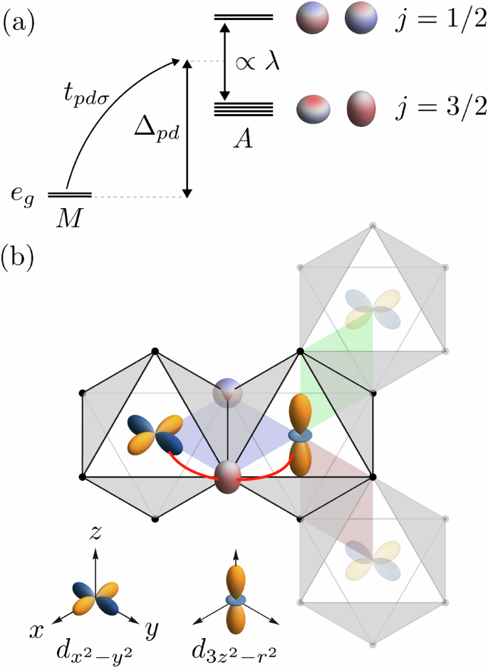
a Virtual hopping process of one hole (or electron) between adjacent M and A sites separated by the charge transfer gap Δ_pd. Large SOC λ on the A site splits the p orbitals into j = 1/2 and j = 3/2 states and is responsible for generating an imaginary spin-dependent hopping. Separation of the d orbital manifold into t_2g and e_g irreducible representations due to cubic crystal field splitting and filled t_2g (not shown) are imposed. Charge densities for the j = 1/2 Kramer’s doublet is shown alongside its label, with the red and blue texture representing spin up and spin-down density, respectively. Two of the j = 3/2 states are plotted alongside their label for j^z = 1/2 (left) and j^z = 3/2 (right). b Honeycomb lattice formed from M sites, located at the center of each octahedral cage of A sites. Orbitals are centered at the atomic sites; positive and negative lobes are encoded by orange and blue, respectively. The x (red), y (green) and z (blue) bonds are represented as transparent planes and are related by the honeycomb C₃ symmetry. Red lines represent a hole or electron hopping (∝ t_pdσ) between M and A sites; together, these paths provide an inter-orbital bridge via the ligand between sites M_i and M_j. Only these two paths are shown for simplicity.

Full size image

Motivated by this seminal work, Yao and Lee proposed a generalized version of the Kitaev model, referred to as the Yao-Lee (YL) model, expressed as²⁷

where S and T represent spin and pseudospin, respectively. The model emerges as a low-energy effective Hamiltonian on the star lattice, whose ground state is a Z₂ spin liquid. Yao and Lee solved the model by decomposing the spin and pseudospin into two Majorana fermions, resulting in three species of gapless Majorana fermions coupled to a ({{mathbb{Z}}}_{2}) gauge field. By Lieb’s theorem, the ground state lies in the zero flux sector, yielding a Dirac dispersion for the Majorana fermions. It exhibits spin-1 fermionic excitations, a zoo of vison crystal phases, and in the presence of an external field, non-abelian spinons^27,28,29. Due to the additional degree of freedom, this model is robust to more perturbations than the original Kitaev model^{30,31,32,33,34}, making it an attractive alternative candidate.

While fascinating, identifying the microscopic mechanisms that give rise to such interactions remains a significant challenge. When mapped onto a honeycomb lattice, additional degrees of freedom may arise from orbital fluctuations. However, it is well-established that when orbital fluctuations play a role in exchange processes, models like the Kugel-Khomskii (KK) model, characterized by a product of spin-Heisenberg and orbital-Heisenberg interactions³⁵, or the compass model³⁶ typically emerge. This raises the question of how to generate bond-dependent Kitaev interactions acting on either spins or orbitals, while retaining the Heisenberg interaction for the other.

To appreciate the difficulty inherent in this problem, it is essential to recognize that the Kitaev interaction requires orbital changes through hopping, which depend on the bond direction^11,12,13,20. Therefore, the origin of the Kitaev interaction lies in the orbitals, which manifest as pseudospin bond-dependent interactions via SOC. If we treat orbitals as a separate degree of freedom from spins, the result is either the KK or compass model. Conversely, introducing the SOC required for Kitaev interactions entangles spin and orbital degrees of freedom, eliminating the possibility of treating them separately, as is necessary for generating the YL model.

Here, we outline how to overcome this challenge, and present a roadmap for generating a YL type interaction on the honeycomb lattice. By leveraging the strong SOC of anions in the exchange process within an edge-sharing structure like the honeycomb lattice, we find an exactly solvable YL-like spin-orbital model, termed flavored-Kitaev model. The key idea is that the spin-orbital model obtained through indirect exchange—via an intermediate anion with strong SOC—between neighboring e_g ions includes the flavored-Kitaev interaction, along with a weaker KK interaction. For the 90° edge sharing lattice such as the honeycomb, interorbital hopping between e_g orbitals is only allowed via the anion, making this exchange process dominate over intraorbital direct exchange.

Utilizing classical Monte Carlo (MC) simulations and exact diagonalization (ED), we map the classical and quantum phase diagrams, revealing a large disordered region that breaks rotational symmetry and encompasses an exactly solvable flavored-Kitaev spin-orbital liquid. Our work offers a microscopic pathway to transition from the traditional KK limit to the bond-dependent flavored Kitaev limit in orbital-fluctuating Mott insulators. We propose that d⁹ or low-spin d⁷ systems, surrounded by heavy ions forming a honeycomb lattice, would serve as promising candidate materials.

Microscopic derivation

We first recall how the KK model arises to make a comparison with the mechanism of the flavored-Kitaev interaction. Consider one electron or hole in two degenerate orbitals at M sites, leading to fluctuations between the two orbitals. To represent the orbitals, we introduce pseudospin-1/2 operators ({T}^{k}=frac{1}{2}{sigma }^{k}) with k = x, y, z, where σ^k are Pauli matrices, such that (leftvert arightrangle) and (leftvert brightrangle) are eigenstates of T^z with eigenvalues ({pm}!frac{1}{2}), respectively. Orbital (m) preserving, intraorbital hopping of electrons between neighboring transition metal (M) sites M_i and M_j,

where t_m is the hopping amplitude, resulting in the low-energy spin and orbital model colloquially known as the KK model^35,37,38,39. The SU(4) Kugel-Khomskii model is a classic example of frustration between degrees of freedom and is given by

where ({J}_{{rm{kk}}}=frac{8{t}_{m}^{2}}{U}) when the direct hopping t_m is the same for the two orbitals. It is characterized by isotropic interactions between nearest-neighbor spin-1/2 (S_i) and pseudospin-1/2 (T_i) degrees of freedom and has been suggested to display a spin-liquid ground state on the honeycomb lattice^{40,41,42,43,44,45}, but it lacks exact solvability.

At this stage, exchange between nearest neighbor M sites will generate pseudospin compass and KK exchange interactions depending on the lattice geometry and relative hopping amplitudes^35,36. The Kitaev interaction is absent. The key missing element is SOC, which enables bond-dependent spin interactions while allowing the other degrees of freedom to behave in a Heisenberg fashion.

Now let us consider a honeycomb lattice of e_g orbitals at M sites, surrounded by edge-shared octahedra of heavy anions (A) with large SOC (λ), as illustrated in Fig. 1. Due to the bonding geometry, indirect interorbital hopping via p-orbital superexchange, which mediates a change in angular momentum, dominates over the direct intraorbital hopping. Large anion SOC on the A site leads to a splitting of the single hole states into j = 1/2 and j = 3/2 manifolds, separated by an energy (frac{3}{2}lambda) as shown in Fig. 1.

After taking into account the SOC on the p-orbitals at A sites, we determine an effective nearest-neighbor hopping between e_g ions by integrating out the ligand p-orbitals. Due to the symmetry imposed by the ideal octahedra and 90° bonding geometry, seen in Fig. 1, only hopping via σ-bonds (t_pdσ) between d– and p-orbitals at M and A sites, respectively, is permitted. Assuming that t_pdσ is much smaller than the charge-transfer gap Δ_pd, the effective hopping between e_g ions at the sites M_i and M_j on a z-bond though the anion p-orbitals is given by,

where ({t}_{{rm{eff}}}=scriptstylefrac{{t}_{pdsigma }^{2}}{4sqrt{3}}left(scriptstylefrac{1}{{Delta }_{pd}-frac{lambda }{2}}-frac{1}{{Delta }_{pd}+lambda }right)), and σ = ±1 for spin up and down respectively. We emphasize that this hopping is only finite with SOC present on the A site, which can be seen explicitly in the expression for t_eff, where interference between different exchange paths results in an exact cancellation when λ = 0.

We determine the exchange interactions using strong-coupling perturbation theory truncated at second-order, assuming that t_eff is small compared to the onsite Coulomb interaction, U. For further details, we refer to the supplementary information (SI) (see Supplemental Material at https://doi.org/10.1038/s41535-025-00744-9 for a derivation of the effective model, details of the numerical simulations, and comparisons of the phases). If the M sites are well-separated such that the dominant exchange process is through the ligands, a strong-coupling expansion yields the final form of the effective spin-orbital model

where (Jequiv frac{8{t}_{{rm{eff}}}^{2}}{U}). The YL-like interaction with spin-1/2 having Kitaev type combined with a Heisenberg orbital interaction (({S}_{i}^{gamma }{S}_{j}^{gamma }otimes {{bf{T}}}_{i}cdot {{bf{T}}}_{j})) is uncovered, along with other interactions. Note that if we perform a two-site sub-lattice transformation on the orbital operators,

the first two terms of the orbital interactions are cast into Heisenberg form, and we obtain

which we dub the flavored-Kitaev interaction. Note that the bond-dependent interaction acts on spins, not orbitals. While there is a negative sign in ({T}_{i}^{y}{T}_{j}^{y}), the ground state is expected to be the same as the YL model. As demonstrated in the SI, the energy spectra obtained via the ED for the YL model and the flavored-Kitaev model are identical up to the 10⁻⁶ decimal place.

It is also noteworthy that in the absence of orbital fluctuations, as in the case of d⁸ (i.e., two electrons or holes in the e_g orbital), the spin interaction becomes a sum of Heisenberg and Kitaev interactions, with the Kitaev term being twice as large as the Heisenberg term. This effect resembles the higher-spin Kitaev interaction mechanism described in ref. ⁴⁶, where the factor of 2 difference originates from the e_g wavefunctions.

Moreover, the full model H_eff given by Eq. (6) exhibits a hidden SU(4) symmetry and can be rewritten as the KK model, Eq. (4) with J_kk = −J < 0 after sub-lattice transformations on the orbital operators (Eq. (7)), and 4-sublattice transformation on the spin operators. This has been shown in the Heisenberg-Kitaev (JK) model to give rise to a hidden SU(2) symmetry after a ({{mathcal{T}}}_{4}) sub-lattice transformation, and can be transformed into a pure Heisenberg form⁴⁷. Importantly, the SU(4) KK model with FM interaction results in an ordered ground state, as we will see in the following sections, in contrast to the spin-orbital liquid reported to appear in the AFM SU(4) model⁴⁰. Interestingly, a model with a similar structure arises from the J = 3/2 states of d¹ compounds in the absence of Hund’s coupling⁴³, however, the composition of the pseudospin operators in terms of electron spin and orbital operators remains unclear, lacking the simplicity and tunability of our model (Eq. (6)) together with the KK interaction.

Taking into account the direct intraorbital hopping process that leads to the KK interaction modifies the coefficients in front of (S_i ⋅ S_j)(T_i ⋅ T_j), S_i ⋅ S_j, and T_i ⋅ T_j. Note that the direct intraorbital hopping generated KK interaction Eq. (4) has the opposite sign, making the overall KK interaction strength weaker. We introduce two parameters α and β to account for the exchange couplings J and J_kk. We study the following model Hamiltonian for the γ = x, y, z bond to understand the impact of other terms to the YL model:

H_eff corresponds to α = 1 and β = 1/4, while the flavored-Kitaev (or YL) and KK limit correspond to α = β = 0 and α → ∞, respectively.

Below we present the classical and quantum phase diagrams, with J ≡ 1, by tuning α and β to understand how the YL limit is connected to the KK limit, followed by the MC and ED methods used to obtain the phase diagrams.

Classical phase diagram

The classical phase diagram of Eq. (9) on a honeycomb lattice as a function of α and β is presented in Fig. 2. We perform classical Monte Carlo simulations by treating the spin and orbital degrees of freedom as vectors with magnitude (frac{1}{2}) in ({{mathbb{R}}}^{3}). We take into account both spins and orbitals by considering a honeycomb bilayer with each layer representing its own degree of freedom, coupled by the quartic interactions in Eq. (9). Details of the cluster geometry and simulation parameters can be found in the SI (see Supplemental Material at https://doi.org/10.1038/s41535-025-00744-9 for a derivation of the effective model, details of the numerical simulations, and comparisons of the phases).

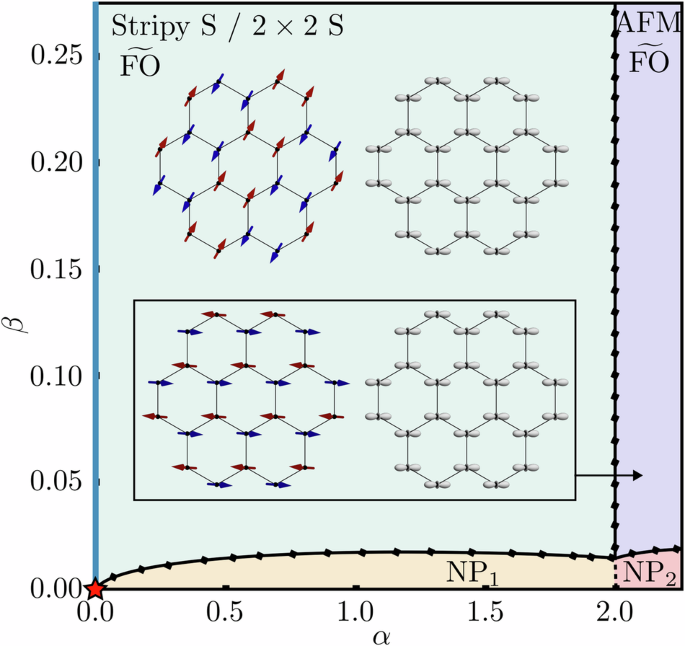
Solid black lines denote interpolated phase boundaries, and square markers denote a small subset of points where the second derivative of the ground state energy was calculated and diverges. Stripy spin / (tilde{FO}) and AFM / (tilde{FO}) orders are shown in the insets. Arrows which are directed in the (+hat{c}) ((-hat{c})) direction are colored red (blue), and black arrows lie within the ab plane. Classical spin/orbital configurations and correlators for nematic phases (NP₁ and NP₂) are shown in the SI. We use a thick blue line to emphasize the spin-disordered line along α = 0, and a red star to represent the classical YL model.

Full size image

Let us first discuss the large β regime. For large β, we find two ordered phases depending on the value of α. The structure of the ordered phases bears a strong resemblance to the phase diagram of the pure JK model on the honeycomb lattice^13,23. In particular, when 0 < α < 2, we have an ordered stripy spin/ferro-orbital ((tilde{FO})) phase and a 2 × 2 spin / (tilde{FO}) phase that is classically degenerate, where the tilde represents the ordering pattern after the T^x/z sublattice transformation, Eq. (7). Spin and orbital configurations for the 2 × 2 spin / (tilde{FO}) order are presented and discussed in more detail in the SI. The red and blue arrows in the inset of Fig. 2 represent the stripy spin order, while the orbital shapes denote ferro-orbital order. When α = 2, there is a second-order transition to the antiferromagnetic (AFM) spin, while the orbital ordering (tilde{FO}) phase remains the same (shown in the bottom inset of Fig. 2), similar to the pure JK model, which undergoes a transition from stripy spin to AFM order when J > 0 and J = −K. This transition is insensitive to the value of β as indicated by a straight transition line in Fig. 2.

For small β, we identify two regions of intriguing phases. To understand the nature of these phases, we compute the structure factors

and the spin-orbital (SO) correlator given by

Both phases display no ordering in the spin and orbital correlators. 〈∑_iS_i〉 = 0, but a higher rank for instance (langle {sum }_{i}{({S}_{i}^{a})}^{2}rangle,ne,0). This suggests that a spin acts like a director with a specific orientation chosen (a-axis in this case, which is perpendicular to one of the honeycomb bonds) like in the nematic phase. For this reason, we will refer them as nematic paramagnetic (NP) phases, denoted by NP₁ and NP₂. The orbitals follow the spin nematic pattern, and the SO correlators show a peak at M and Γ points in NP₁ and NP₂, respectively. The details of the correlators are shown in the SI.

The line α = 0 denoted by the solid blue line in Fig. 2 is a region of particular interest. Along this line, when β = 0, both spins and orbitals are completely disordered, and we represent this point by a red star in Fig. 2, which corresponds to the YL-like spin-orbital liquid limit. As soon as β ≠ 0, the orbitals immediately exhibit (tilde{FO}) order due to the bilinear terms overcoming the frustrated quartic interactions exhibiting a peak in T(Q) at Γ point (see SI), while the spin is disordered. It is interesting that α that effectively includes the Heisenberg interaction, does not lead to a conventional spin or orbital ordered phase, unlike β, which is more detrimental to the disordered spin-orbital limit. The plots for the classical orders and structure factors can be found in the SI.

Quantum phase diagram

The quantum phase diagram is presented in Fig. 3, which was determined with the QuSpin exact diagonalization package; simulation details are included in the SI (see Supplemental Material at https://doi.org/10.1038/s41535-025-00744-9 for a derivation of the effective model, details of the numerical simulations, and comparisons of the phases)⁴⁸. The quantum phase diagram exhibits the same ordered phases as the classical case with the phase boundaries vastly shifted. For large β around 1/4, the transition line between stripy and AFM spin with (tilde{FO}) order occurs at a smaller α, similar to the JK model^13,23. From exact diagonalization, we only find the stripy spin / (tilde{FO}) order, in contrast to the phase diagram obtained classically. This may be due to the limited cluster shape and size of the quantum simulation or quantum fluctuations selecting the stripy order over the 2 × 2 order.

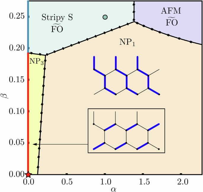
The green dot denotes the ground state of the effective model H_eff corresponding to α = 1 and (beta =frac{1}{4}). NP₁ and NP₃ denote the NP phases in the quantum model that were distinguished by looking at bond-energy correlators shown in the inset. Bonds with lower energy are denoted by dark blue lines. The light blue line at α = 0 for large β denotes a region with no signatures of long-range spin or orbital order. The exactly solvable point is denoted by a red star and exhibits a spin liquid ground state, which extends to β ≈ 0.19 and is emphasized by a thick red line.

Full size image

The disordered regions in the quantum model have extended to a much larger β. A wide regime of the phase space is occupied by NP₁. As in the classical phase diagram, the disordered NP phases both have vanishing bilinear correlators S(Q) and T(Q), indicating disorder. However, these orders spontaneously break the lattice C₃ symmetry, which we show by determining the bond energy correlators ({O}_{ij}^{gamma }=langle {H}_{ij}^{gamma }rangle). The result is plotted in the inset of Fig. 3; bonds with lower energy are denoted by a thick blue line. The lower energy bonds form a chain in NP₁. Additionally, a new nematic phase, NP₃ emerges for smaller α regime. Unlike NP₁, the lower energy bonds form a dimer, implying that the relative difference between the two NP phases is independent of the ED cluster shape.

When α = 0 and β = 0, represented by a red star in Fig. 3, the quantum model belongs to a large class of exactly solvable models³¹. At this point, the model can be cast into quadratic form by writing the spin and orbital degrees of freedom in terms of Majorana fermions, ({S}_{i}^{alpha }=-frac{i}{4}{epsilon }^{alpha beta gamma }{c}_{i}^{beta }{c}_{i}^{gamma }) and ({T}_{i}^{alpha }=-frac{i}{4}{epsilon }^{alpha beta gamma }{d}_{i}^{beta }{d}_{i}^{gamma }). Interestingly, ED suggests that the spin liquid phase survives for a large window of β along the α = 0 line denoted by the red line in Fig. 3, since no discontinuities in the ground state energy or its derivatives were observed. This can be contrasted with the classical phase diagram, where this line collapses into a single point, suggesting the phase is stabilized by quantum fluctuations.

When α = 0 and β ≳ 0.19 indicated by the solid blue line in Fig. 3, a phase transition to another disordered phase is observed. In this phase, there is no evidence of long-range ordering in both spin and orbital degrees of freedom, unlike the classical model, which orders in the orbital degree of freedom. However, this discrepancy may be due to finite-size effects. It is worth noting that nematicity was observed in the SU(4) KK model with antiferromagnetic interaction⁴⁰, but it disappears as the system size increases. The finite-size effects on the NP phases also warrant further investigation.

As mentioned, when α = β = 0, our Hamiltonian maps to the exactly solvable flavored-Kitaev model, which is similar to the YL model, but there are two important differences. The bond-dependent Ising interaction appears on the spin, not on the orbitals, and the orbital interaction is not the Heisenberg type, but is XXZ-like, ({T}_{i}^{x}{T}_{j}^{x}+{T}_{i}^{z}{T}_{j}^{z}-{T}_{i}^{y}{T}_{j}^{y}). In terms of Majorana fermion operators, ({S}_{i}^{alpha }=-scriptstylefrac{i}{4}{epsilon }^{alpha beta gamma }{c}_{i}^{beta }{c}_{i}^{gamma }) and ({T}_{i}^{alpha }=-frac{i}{4}{epsilon }^{alpha beta gamma }{d}_{i}^{beta }{d}_{i}^{gamma }), the model is then written as ({mathcal{H}}=frac{1}{8}{sum }_{langle ijrangle }{hat{u}}_{ij}(i{d}_{i}^{x}{d}_{j}^{x}+i{d}_{i}^{z}{d}_{j}^{z}-i{d}_{i}^{y}{d}_{j}^{y})) where ({hat{u}}_{ij}=-i{c}_{i}^{gamma }{c}_{j}^{gamma }). This implies that it is the orbitals that fractionalize into gapless Majorana fermions in the background of the zero-flux sector composed of the c Majoranas. Note that the e_g orbitals transform like pseudospins, and T_x and T_z carry quadrupolar moments, while T_y carries an octupolar moment; ({T}_{x}=1/(2sqrt{3}){Q}_{{x}^{2}-{y}^{2}},{T}_{y}=1/(3sqrt{5}){O}_{xyz},{T}_{z}=1/(2sqrt{3}){Q}_{3{z}^{2}-{y}^{2}}). A complex fermion operator can then obtained by combining ({d}_{i}^{z}) and ({d}_{i}^{x}) Majorana fermions, ({f}_{i,y}=({d}_{i}^{z}-i{d}_{i}^{x})/2), implying fermionic octupolar excitations in the ground state.

It is also worth drawing comparisons to models such as the spin-1/2 KΓ model in a finite field and the spin-1 bi-linear bi-quadratic Kitaev (BBQ-K) model, which exhibit nematic orders bordering the spin liquid region^49,50,51,52. In particular, for the KΓ model, as the Γ interaction is increased in a finite field along the [111] direction, there is a transition between two nematic phases with the same bond-energy correlators as our NP₃ and NP₁ phases. The BBQ-K model also undergoes a transition, at a large enough bi-quadratic interaction, from the Kitaev spin-liquid through a nematic phase before entering an ordered stripy spin phase (see Fig. 3 of ref. ⁵²). A similar sequence of transitions occurs in our model, as shown in Fig. 3, when β ≈ 0.19.

There are many exciting avenues for future exploration. One possible direction is to identify microscopic mechanisms to tune the system toward the exactly solvable point or to expand its stability in phase space. For instance, exchange processes such as cyclic and two-hole exchanges, which are beyond the scope of the current study, will introduce additional symmetry-allowed interactions and may reduce some unwanted interactions. For example, the compass interaction on orbital degrees of freedom can be present. However, the flavored-Kitaev spin-orbital liquid is protected by the Z₂ flux gap inherent to the spin interaction with the Kitaev-type interaction. Thus, as long as the orbital compass interaction is small, the spin-orbital liquid is expected to be stable. Investigating these interactions and their impacts on the flavored-Kitaev spin-orbital liquid’s stability window would be valuable.

In terms of material candidates, d⁹ ions on a honeycomb lattice with edge-sharing ligands with strong SOC present a promising option. For example, the compound Ba₃CuSb₂O₉ consists of honeycomb layers of Cu²⁺ atoms carrying a d⁹ configuration. Remarkably, this compound exhibits no Jahn-Teller distortions, preserving the e_g doublet, and shows no evidence of long-range ordering down to zero temperature⁵³. While the SU(4) spin-orbital liquid, represented by the KK model with antiferromagnetic interaction, was proposed⁴⁰, the flavored Kitaev interaction is also allowed. Exploring its interplay with the KK interaction in this candidate material presents an interesting direction for future research. d⁷ compounds (such as Co²⁺) are another possibility, but due to the strong Hund’s coupling, achieving a low-spin state, one electron in the e_g orbital, while keeping the octahedra crystal field symmetry may be challenging. We hope that our theory will inspire further studies on extended models and the search for flavored-Kitaev spin-orbital liquid candidates.

In summary, we present the first microscopic theory that links the extensively studied KK model to the exactly solvable YL-like limit, referred to as the flavored-Kitaev model. We demonstrate that d⁹ ions (or d⁷ ions with sufficiently large cubic crystal field splitting, leading to a low spin state) surrounded by heavy ligands with SOC coupling are positioned near large swaths of nematic phases that engulf an exactly solvable spin liquid point, verified through both classical and quantum simulations. Our work serves as a starting point for the search for materials that exhibit this new class of flavored-Kitaev spin-orbital liquid featuring fermionic octupolar excitations. Given the limitations of the current methods—small size ED and classical Monte Carlo—employing other numerical techniques, such as variational methods and density matrix renormalization group, to explore the extended Kitaev-Yao-Lee model would be valuable for future studies.

The phase diagrams were computed using classical Monte Carlo simulations and exact diagonalization. To encode both degrees of freedom, we considered a honeycomb bilayer with one lattice representing spin and another representing orbitals. We determined the phase boundaries with both methods by identifying divergent behavior in ∂²E_GS/∂α² and ∂²E_GS/∂β², where E_GS is the energy of the groundstate.

Classical Monte Carlo simulations were carried out using ClassicalSpinMC.jl (www.github.com/emilyzinnia/ClassicalSpinMC.jl), treating the spin and pseudospin degrees of freedom as vectors with magnitude (frac{1}{2}) in ({{mathbb{R}}}^{3}). We computed the classical phase diagram using a 528-site honeycomb bilayer, generated by a 12 × 12 triangular lattice with 4 sites per unit cell. Two sites in the unit cell belong to the spin layer, and two belong to the orbital layer, and they are coupled by the quartic interactions between the degrees of freedom. For each point in the phase diagram, we used an adaptive metropolis simulated annealing algorithm⁵⁴ with 10⁵ thermalization steps cooled down to a temperature of 10⁻⁷. During thermalization, 10 overrelaxation sweeps (also known as microcanonical sweeps)⁵⁵ were performed for every Metropolis sweep for faster convergence. The spins were then deterministically updated for 10⁶ sweeps such that they aligned towards the local field⁵⁶.

Exact diagonalization was performed using the QuSpin python package⁴⁸, with the Lanczos algorithm. We computed the quantum phase diagram using a 24 site honeycomb bilayer (12 sites for each degrees of freedom), with periodic boundary conditions. Cluster details can be found in the supplementary information (SI).