Modeling critical dosing strategies for stromal-induced resistance to cancer therapy

Introduction
The ability of cancer therapies to enhance the development and outgrowth of resistant tumor subpopulations is becoming increasingly recognized as an important contributor to therapeutic failure. In the context of both bacterial and cancer cell populations, it has been observed that drug-induced stress can lead to elevated mutation rates, via switching to less reliable DNA repair mechanisms1 or elevating levels of reactive oxygen species which can induce oxidative DNA damage. In the setting of non-small cell lung cancer cells, Sharma and colleagues established the existence of a drug-tolerant phenotype that is transiently acquired and relinquished at low frequency by individual cells within the population, with a pathway to acquiring stable resistance conferred in the presence of a targeted therapy2. Similarly, Shaffer et al. demonstrated that profound transcriptional variability within human melanoma cells can lead to transient drug-resistant phenotypes, which can then be epigenetically reprogrammed to stably resistant states through the addition of drug3. In all cases, the opposing drug-induced resistance costs vs tumor-reduction benefits suggest that careful selection of dose and timing may be required for designing optimal therapeutic strategies and reducing therapeutic failures.
One common mechanism of drug-induced resistance is the remodeling of the tumor microenvironment (TME) to create protective niches where cancer cells can survive therapy or resistant cells can thrive (e.g., ref. 4), or therapy-induced plasticity wherein tumor cells transition into more drug-tolerant phenotypic states in the presence of therapy5. Therapy can induce tumor cells or stromal cells within the TME to secrete signaling factors that protect cancer cells from the effects of therapy. For example, cancer-associated fibroblasts (CAFs), the most abundant stromal cell population within the TME, have been observed to secrete signaling factors that protect tumor cells from the cytotoxic effects of cetuximab in colorectal cancer (CRC)6. Targeted therapy with BRAF, ALK, or EGFR inhibitors was shown to induce changes to the cancer cell secretome that stimulate the outgrowth of drug-resistant cancer cells in melanoma and lung adenocarcinoma cells7. In addition, drug-induced enrichment of a subpopulation of fibroblasts promoted chemoresistance in breast and lung cancer models through cytokine-mediated (IL-6 and IL-8) cancer stem cell survival8.
There has been substantial recent interest in the development of mathematical models of therapy-induced resistance, which is increasingly acknowledged as a major driver of treatment failure in cancer9,10,11,12,13,14,15,16,17,18,19. For example, Pisco et al.9 investigated the induction of multi-drug resistance in HL60 leukemic cells following treatment with vincristine through a combination of experiments and mathematical modeling. More recently, Gevertz et al. developed a model of drug-induced resistance and fit this model to in vitro data, and then applied techniques of optimal control to discover optimal dosing strategies in light of this phenomenon10. In this work, we focus on developing mathematical models for the general scenario in which a stromal cell population secretes signaling factors that protect cancer cells from the effects of therapy, in a drug-dependent manner. There have been some mathematical models developed previously for designing optimal therapy strategies in light of increased drug-induced mutation rate, considered in ref. 1 and references therein. Some modeling works have specifically investigated intra- and intercellular signaling of cancer and stromal cells that induce a transition to the activated fibroblast state and in return influence tumor progression20. The authors in ref. 21 consider a cell-level model for sensitive and resistant melanoma cells and associated fibroblasts under treatment with BRAF and FAK inhibitors. They briefly address the question of treatment with simple on/off periods of drug administration, allowing the cancer cells to re-sensitize during treatment breaks. This idea is further studied in a recent preprint, where the authors investigate a spatially structured model for interacting cancer cells, stromal cells, and blood vessels22. Moreover, the idea of adaptive treatment that alters protocols based on the tumor’s response and allows for the heterogeneous cancer cell population to re-sensitize has been explored computationally in ref. 23. In a recent paper24, the impact of stochastic fluctuations on adaptive therapy design is addressed by a stochastic optimal control approach. In our work, we build upon these studies to investigate optimization of treatment strategies (with regards to administration time and dose) in relation to threshold drug concentrations for triggering responses in both cancer and stromal cells.
Our approach to optimizing treatment protocols for drug-induced resistance through increased growth factor secretion by stromal cells is structured as follows: We first focus on the short-term dynamics of the system to predict effective drug concentrations (in terms of inducing tumor reduction), based on the specific composition of the microenvironment (see the section “Drug concentration thresholds for tumor reduction”). Moreover, we investigate potential combination treatment that targets the stromal cells and their growth factor secretion dynamics by studying the sensitivity of the treatment outcome and effective concentrations to the variation of a number of system parameters (see the sections “Combination therapy—targeting stromal cells”, “Combination therapy—targeting stromal drug response”, “Combination therapy—targeting growth factor efficacy”). Based on the acquired knowledge of these short-term dynamics, we suggest strategies for treatment optimization, considering the long-term outcome of the system. We study periodic drug administration and drug decay, varying both the administered drug concentration and break time between administrations (“Treatment optimization for long-term outcomes”). This general model is motivated by the specific application of CRC cells interacting with CAFs and the observations in ref. 6. In this system, under treatment with the EGFR inhibitor cetuximab, CAFs demonstrate increased EGF secretion which then induces partial drug resistance. We consider this specific scenario as a case study in “Application: CRC–CAF interactions”, where we investigate the advantages of combination therapy with EGF-blockers and different protocols for single- and multi-drug treatment. This mathematical modeling framework, guided by experimental and/or clinical observations, contributes to a better understanding of the microenvironment’s contributions to drug-induced resistance and clinical strategies for overcoming them.
Results
Mathematical model
We first propose a general model for drug-induced resistance through environmental remodeling by a stromal cell population. In particular, consider a population of cancer cells C and a population of stromal cells S in the tumor microenvironment (such as CAFs). The stromal cells secrete a growth factor G that induces partial drug resistance in the cancer cells, and this secretion rate as well as the cancer growth rate may be dependent on the drug concentration D. The state of the system at time t ≥ 0 is then described by ((C(t),S(t),D(t),G(t))in {{mathbb{R}}}_{+}^{4}), where C(t) and S(t) are considered as numbers of cells and D(t) and G(t) as concentrations. Mathematically, we describe the dynamics of this system using the following system of ordinary differential equations; a schematic is provided in Fig. 1a.

a Interaction diagram summarizing the dynamics of the general model in Eq. (1). Each solid or dashed arrow corresponds to an event that changes the system state. Dotted arrows mark the influence of D and G on the dynamics of C and S. Created in BioRender https://BioRender.com/i95h85832. b Dose–response curve for the cancer cell growth rate rC(D, G), depending on drug concentration D, for a fixed low growth factor concentration G (solid line). Increasing G shifts the response curve right (dashed line). c Drug concentration for 50% efficacy D50(G) (dose–response curve inflection point), depending on the growth factor concentration G. d Equilibrium growth factor concentration (overline{G}(S,D)), depending on drug concentration D, for fixed number of stromal cells S.
Here, rC is the exponential net growth rate of cancer cells, dependent on the drug and growth factor concentrations and rS is the exponential net growth rate of the stromal cells, which can depend on the drug concentration. In addition, bG is the rate of growth factor secretion, which may be dependent on the drug concentration and number of stromal cells. Lastly, dD and dG denote the decay rates of the drug and secreted growth factor, respectively. Here, we have assumed unrestricted exponential growth for cancer and stromal cells, reflecting a regime in which resources are not limited. Note that this model could easily be extended to a stochastic (agent-based) Markov process to study stochastic events such as extinction in small population settings.
To study treatment resistance, many models distinguish between sensitive and resistant cancer cells and introduce either a reversible phenotypic switching mechanism between these two states or a non-reversible mutation. In the case of growth factor-induced resistance, the presence of many receptors that can bind to either drug or growth factor molecules and the relatively quick (un)binding dynamics result in more of a continuum of cancer cell states that display different dynamics, based on the current drug and growth factor concentration and the corresponding equilibrium receptor state. We therefore choose to consider a continuum of drug-resistance phenotypes, i.e., to have the mean growth rate rC of the cancer cell population depend on the drug and growth factor concentrations in a continuous way.
Dependence of cancer growth on drug and growth factor concentration: The dependence of the cancer cell growth rate rC(D, G) on the drug concentration D is modeled by a classic Hill function (dose–response curve), as depicted in Fig. 1b. We set
The increased growth rate of the cancer cells under increasing growth factor concentration is reflected in the varying inflection point D50(G) of the response curve, which marks the drug concentration of 50% efficacy. In particular, an increasing growth factor concentration G shifts the Hill function curve to the right (see Fig. 1b). This increase of D50(G) under increasing growth factor concentration is modeled as a logistic function
where (hat{G}) is the inflection point. It roughly corresponds to the threshold growth factor concentration to induce cancer cell drug resistance (see Fig. 1c). These forms of dependence are consistent with our experimental dataset on CRC–CAF interactions (see sections “Application: CRC–CAF interactions” and “Dose–response curve and D50”).
Note that if ({r}_{C}^{min },<,0,<, {r}_{C}^{max }), the critical drug concentration Dcrit(G) at which the growth rate changes sign (i.e., rC(D, G) <0 if and only if D > Dcrit(G)) can be calculated as
Dependence of growth factor secretion on drug concentration: In vitro experiments with stromal cells indicate that an equilibrium growth factor concentration (overline{G}) is achieved quickly by secretion and remains stable at least over the course of multiple days (see “EGF secretion and varying CAF number/type”). To depict the dependence of this equilibrium concentration on the drug concentration, we model (overline{G}(S,D)) as a logistic function
where ({G}^{max }(S)) is the maximal concentration (dependent on the number of stromal cells S) and (hat{D}) is the inflection point (see Fig. 1d). The latter roughly corresponds to the threshold drug concentration to induce increased growth factor secretion of stromal cells.
To study the short-term dynamics of cancer and stromal cells responding to drug treatment, we simply assume the growth factor concentration to be in equilibrium, while we use a dynamics growth factor secretion and degradation at rates bG(S, D, G) and dG to model long-term dynamics. Since we consider relatively fast growth factor secretion and degradation, e.g compared to drug degradation, in this paper, the growth factor secretion still follows closely along its equilibrium and the exact form of the secretion rate is not too important. We refer to “Secretion and degradation for treatment with breaks” for details.
Impact of stromal content level on growth factor concentration: The concentration of growth factors inducing drug resistance of cancer cells may be dependent on the level of stromal content in the tumor. We model the impact of the stromal content level on the the maximal growth factor concentration ({G}^{max }(S)) in two ways: We consider (i) a dose-dependence phenomenon in which the maximal growth factor concentration depends linearly on stromal population levels via slope k4
reflecting a fixed increase in the maximal growth factor concentration per stromal cell. Alternatively (ii), as long as there is any stromal presence, a constant maximal growth factor concentration is achieved,
We investigate both possibilities in this work; experimental observations of the CRC-CAFs system are consistent with the second version (see “EGF secretion and varying CAF number/type”).
Effective drug concentrations for short-term dynamics
The success of therapy—in terms of reducing the cancer growth rate in response to an administered drug dose—is dependent on complex interactions between drug, drug-dependent growth factor secretion by stromal cells, and treatment effect on cancer cells. In our first set of investigations, we make several simplifying assumptions to identify regimes of effective drug concentration thresholds and combination strategies to achieve tumor reduction on short time scales, e.g., initial response at the start of treatment. Recognizing that initial tumor reduction may not always correspond to optimal long-term dynamics, however, we will return to the more complicated model (1) to address longer time spans and the option of treatment with breaks in “Treatment optimization for long-term outcomes”.
Simplified model for short-term dynamics: To model the initial treatment response, for the remainder of this section, we assume that drug decay is negligible and just set D(t) ≡ D(0) as the constant concentration that was initially administered. To reflect a much slower-growing stromal cell population than cancer cell population, we also assume rS(D) to be very small or even rS(D) = 0, which entails S(t) ≡ S(0). Finally, as discussed in “EGF secretion and varying CAF number/type”, the CRC experiments demonstrate that the stromal-cancer cell interactions result in a relatively stable concentration of growth factors. We hence set (G(t)equiv overline{G}(S(0),D(0))) as a constant concentration, depending on the constant number of stromal cells and drug concentration. These assumptions are motivated by multi-day experiments performed on colorectal cancer cells interacting with CAFs under treatment with cetuximab; this example is explored in detail in “Application: CRC–CAF interactions”. All of the above assumptions result in the simplified model
which we apply to study initial tumor response to single and combination therapies throughout this section.
Drug concentration thresholds for tumor reduction
Figure 1b in the previous section only depicts the cancer growth rate in response to an increasing drug concentration D for a fixed growth factor concentration G. However, in the more realistic setting where the growth factor concentration depends on the current drug concentration, the more clinically relevant quantity is the effective growth rate of cancer cells within their microenvironment. To find this quantity and determine whether an administered drug concentration Da is successful, one needs to follow three steps:
-
1.
Determine the equilibrium growth factor concentration (overline{G}(S,{D}_{a})) that is induced by the drug’s impact on growth factor secretion by stromal cells. This fixes the corresponding tumor dose–response curve.
-
2.
Use this dose–response curve to determine the corresponding critical drug concentration ({D}_{{rm{crit}}}(overline{G}(S,{D}_{a}))) that is needed to induce a negative growth rate.
-
3.
Compare the administered drug concentration to this induced critical concentration. If the latter is smaller, i.e ({D}_{{rm{crit}}}(overline{G}(S,{D}_{a})),<,{D}_{a}), the induced growth rate is negative, leading to tumor reduction. Otherwise, it is positive and therapy at this administered drug concentration does not control tumor burden.
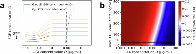
Figure 2a, b visualizes this three-step procedure for two different administered drug concentrations—one corresponding to successful treatment (({D}_{a}^{1})) and one corresponding to failed treatment (({D}_{a}^{2})). Figure 2c directly plots the critical drug concentration ({D}_{{rm{crit}}}(overline{G}(S,{D}_{a}))) as a function of the administered drug concentration Da and Fig. 2d shows the corresponding effective cancer growth rates ({r}_{C}({D}_{a},overline{G}(S,{D}_{a}))). The parameters chosen to generate the plots in this section are summarized in Table 1 in “Application: CRC–CAF interactions”.
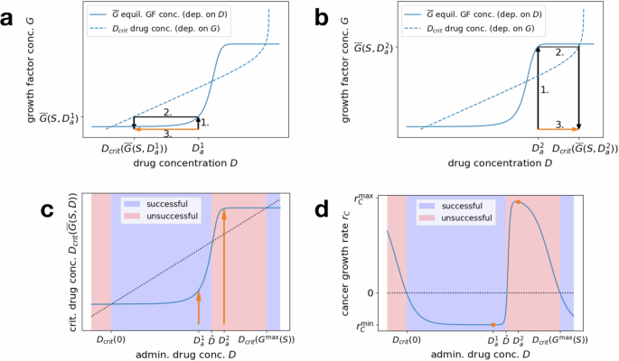
a, b Equilibrium growth factor concentration (overline{G}(S,D)), depending on the drug concentration D (solid line), and critical drug concentration Dcrit(G), depending on the growth factor concentration G (dashed line, axes flipped). To determine the critical concentration induced by an administered drug concentration Da, find the induced equilibrium growth factor concentration (overline{G}(S,{D}_{a})) (1.) and then the corresponding critical drug concentration ({D}_{{rm{crit}}}(overline{G}(S,{D}_{a}))) (2.). Combining these steps yields the orange arrows that compare the administered and corresponding critical drug concentrations (3.). a Successful therapy, where the administered drug concentration ({D}_{a}^{1}) is higher than the critical concentration ({D}_{{rm{crit}}}(overline{G}(S,{D}_{a}^{1}))) corresponding to its induced microenvironment. b Failed therapy, where the administered drug concentration ({D}_{a}^{2}) is lower than the critical concentration ({D}_{{rm{crit}}}(overline{G}(S,{D}_{a}^{2}))) corresponding to its induced microenvironment. c Direct mapping of administered drug concentration Da to the corresponding critical drug concentration ({D}_{{rm{crit}}}(overline{G}(S,{D}_{a}))) (combining the steps of (a, b)). Successful treatment is characterized by the Dcrit line falling below the diagonal (blue), while unsuccessful treatment corresponds to the line lying above the diagonal (red). The windows of (un)successful concentrations are bounded by the approximate thresholds Dcrit(0), (hat{D}), and ({D}_{{rm{crit}}}({G}^{max }(S))). Arrows correspond to the two example concentrations ({D}_{a}^{1}) and ({D}_{a}^{2}) from (a, b). d Direct mapping of administered drug concentration Da to the corresponding cancer cell growth rate ({r}_{C}({D}_{a},overline{G}(S,{D}_{a}))). Successful (rC < 0) and unsuccessful (rC > 0) drug concentration windows are marked as in (c). Orange dots correspond to the two example concentrations ({D}_{a}^{1}) and ({D}_{a}^{2}) from (a, b).
The above considerations allow us to find the minimal drug concentration that induces any negative growth rate for the cancer cells (very close to zero). For most applications, it is however more relevant to push the growth rate below a certain (strictly negative) value so that the tumor size actually decreases and the cancer cells eventually die out, rather than just preventing the tumor from growing. Note that this question can be addressed in exactly the same way. Instead of investigating the critical concentration Dcrit at which the growth rate hill function changes sign, we could have also chosen to study a general
for ({r}_{C}^{min },<, r ,<,{r}_{C}^{max }), the concentration at which the growth rate first drops below r. Studying intersections of this function with the equilibrium secreted growth factor concentration allows us to determine the minimal drug concentration to keep the cancer growth rate below a certain threshold r.
Stromal content impacts the therapeutic window: Interestingly, the success of treatment can exhibit a nonmonotonic behavior, as shown in Fig. 2, where an increase in the drug concentration does not necessarily lead to a better treatment outcome. Eventually, for a high enough administered drug concentration, the cancer growth rate becomes negative. This is due to the fact that, for any fixed stromal cell population S, the drug dose D eventually surpasses the critical drug concentration corresponding to the maximal secreted growth factor concentration, i.e., eventually (D,>,{D}_{{rm{crit}}}({G}^{max }(S))). However, if certain relations between the involved parameters are satisfied, it is possible to have multiple fixed points ({D}_{{rm{crit}}}(overline{G}(S,D))=D), i.e., multiple sign changes of ({D}_{{rm{crit}}}(overline{G}(S,D))-D), corresponding to multiple switches between positive and negative growth rates as the administered drug concentration increases. In particular, this can lead to a window of lower drug concentrations inducing negative growth rates, followed by a window of intermediate concentrations that lead to therapy failure, before reaching a threshold above which all concentrations are successful.
The intuition for this nonmonotonic behavior is explained as follows: consider the inflection point (hat{D}) of the growth factor secretion function. For drug concentrations below this value, the stromal cells secrete lower amounts of growth factor and hence (overline{G}approx 0). For concentrations above (hat{D}), the growth factor secretion is activated and quickly approaches its maximum, i.e., (overline{G}approx {G}^{max }(S)). If
there is a window of drug concentrations ([{D}_{{rm{crit}}}(0),hat{D}]) where the increased growth factor secretion by the stromal cells has not been triggered yet but the drug concentration is higher than the critical concentration corresponding to no growth factor. This induces a negative cancer growth rate. If additionally
then there is a window of drug concentrations ([hat{D},{D}_{{rm{crit}}}({G}^{max }(S))]) where the maximal growth factor concentration is reached but the drug concentration is still below the critical concentration corresponding to this growth factor regime, hence inducing a positive cancer growth rate. These three concentration thresholds defining the windows for successful or unsuccessful treatment are visualized in Fig. 2c, d.
Note that these heuristics essentially assume the growth factor secretion function to be a step function, jumping from 0 to ({G}^{max }(S)) at (hat{D}). This is only a good approximation for steep slopes k3; hence criteria (10) and (11) become less accurate for lower values of k3 (as seen in Fig. 2c, d, where the proposed thresholds do not exactly match up with the fixed points of ({D}_{{rm{crit}}}(overline{G}(S,cdot )))).
Combination therapy—targeting stromal cells
In our model, stromal cells influence the cancer treatment response through the secretion of growth factors. We focus here on analyzing the case in which there is a fixed increase in the maximal growth factor concentration per stromal cell, as in Eq. (6). Here, the maximal growth factor concentration depends linearly on S through ({G}^{max }(S)={k}_{4}cdot S). Since the presence of this growth factor inhibits the effect of the drug on cancer cells, we explore the notion of targeting the stromal cell population in a combination therapy approach. Mathematically, this corresponds to decreasing (or generally changing) the number of stromal cells S ≡ S(0) in Eq. (8). Since we only consider the short-term effects of treatment in this section, the effects of the combination therapy—as well as those in the following sections—are assumed to be static, just as the primary drug concentration D. When considering the long-term dynamics of combination treatment (as we do for the application of colorectal cancer cells in “Long-term treatment”) the secondary treatment would be modeled as an additional dynamic drug concentration and the system would move within the parameter spaces that are explored below.
As can be seen in Fig. 3a with the series of orange lines, decreasing the number of stromal cells pushes down the line corresponding to the secreted equilibrium growth factor concentration. In particular, the maximal growth factor concentration ({G}^{max }(S)) decreases proportionally with S, while the threshold drug concentration (hat{D}) for switching from the low growth factor to the high growth factor regime remains the same (no horizontal shift). This extends the range of drug concentrations corresponding to a negative cancer growth rate regime and in particular lowers the minimal drug concentration necessary to induce a negative cancer growth rate. Eventually, for low enough cell numbers, it is even possible to eradicate the window of intermediate drug concentrations for which the treatment is unsuccessful, effectively eliminating this microenvironmental pathway to resistance for most drug concentrations. Referencing “Drug concentration thresholds for tumor reduction”, this is the case when S is small enough such that ({D}_{{rm{crit}}}({G}^{max }(S))) drops below (hat{D}).
Figure 3b visualizes the same effects in a heat map plot, depicting the growth rate of the cancer cells depending on the number of stromal cells S and the drug concentration D. We can observe that nothing changes for the effects of very high drug concentrations. This is the case because of our function for D50(G), which eventually levels off to ({D}_{50}^{max }) for high G. Whenever the administered drug concentration D is higher than the critical dose Dcrit corresponding to this ({D}_{50}^{max }) (i.e., to the most right-shifted dose–response curve), then the cancer growth rate is negative, independent of the composition of the microenvironment.
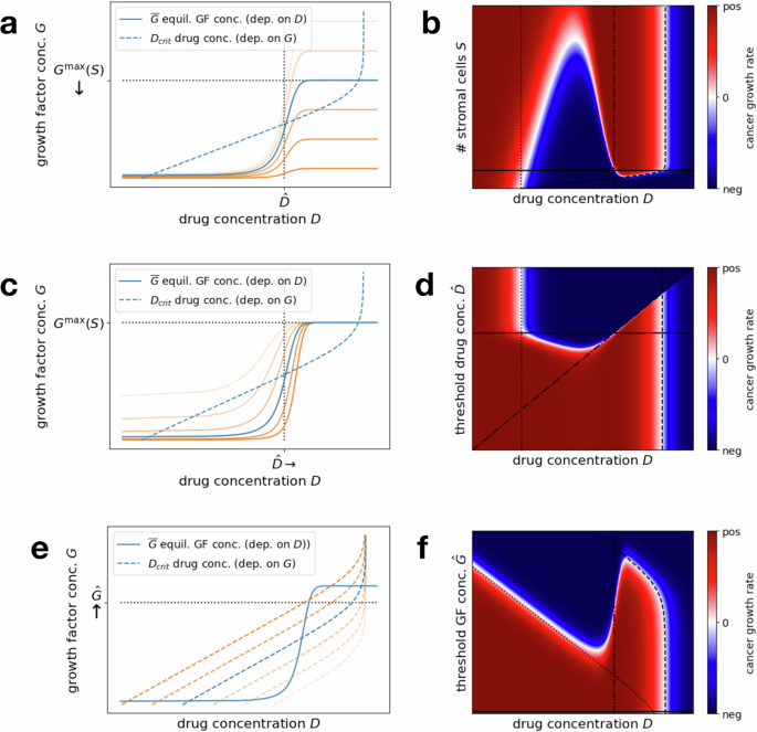
Left panels: Plots as in Fig. 2a, which allow to compare an administered drug concentration Da to the critical drug concentration Dcrit corresponding to its induced growth factor concentration (overline{G}(S,{D}_{a})). Crossings of solid and dashed lines mark the windows of successful and unsuccessful drug concentrations. Blue lines correspond to the original regime while intensifying orange lines depict increasing the efficacy of combination treatment (decreasing stromal cell numbers, stromal drug response or growth factor efficacy). Right panels: Heat maps showing the cancer growth rate for varying drug concentrations D and stromal cell numbers S, threshold drug concentration (hat{D}), or threshold growth factor concentration (hat{G}). Red areas correspond to failed treatment, i.e., positive cancer growth rates, blue areas to successful treatment, i.e., negative cancer growth rates. White areas correspond to a sign change in the growth rate and the black lines mark the original regime (solid), varying Dcrit(0) (dotted) and ({D}_{{rm{crit}}}({D}^{max }(S))) (dashed) and (hat{D}) (dashdotted). a, b Targeting stromal cell numbers S. c, d Targeting stromal drug response, in terms of the threshold drug concentration (hat{D}). e, f Targeting growth factor efficacy, in terms of the threshold growth factor concentration (hat{G}) for a cancer cell response.
Note that, at least under the assumption of a homogeneous cell population, lowering the secreted growth factor concentration by decreasing k4 (i.e., lowering the maximal secreted growth factor concentration per stromal cell) or neutralizing a certain percentage of growth factor molecules through growth factor-blockers would have the same effect as decreasing the number of stromal cells. Both S and k4 enter the function for (overline{G}(S,D)) in a linear fashion through ({G}^{max }(S)). Similarly, neutralizing a given percentage of growth factor molecules yields a linear factor decreasing the concentration of effective growth factor.
Combination therapy—targeting stromal drug response
Another possible target for combination therapies is to decrease the stromal sensitivity to the drug. In contrast to the previous section, this might not decrease the maximal secreted growth factor concentration ({G}^{max }(S)) but rather increase the threshold drug concentration (hat{D}) for switching from the low growth factor to the high growth factor regime. For example, if the drug interacted with stromal cells by binding to a different receptor than the receptor on the cancer cells, there might be a way to (partially) block this receptor specifically. As a consequence, a higher drug concentration would be required to trigger a response in the stromal cells (increasing growth factor secretion), while the cancer cells’ response to the drug remains unchanged. Another approach would be to reprogram cancer-associated stromal cells to a more normal-like state where they may be less sensitive to the drug25.
We explore the effects of varying the threshold parameter (hat{D}) on the short-term dynamics in Eq. (8). As seen in Fig. 3c, increasing (hat{D}) extends the window of lower drug concentrations leading to a successful therapy outcome. This is due to the fact that the upper bound of this window essentially corresponds to (hat{D}) itself, as discussed in “Drug concentration thresholds for tumor reduction”. It is even possible to fully get rid of the opposing window of intermediate drug concentrations corresponding to failed treatment if (hat{D}) surpassed the minimal successful dose corresponding to the highest possible growth factor concentration ({D}_{{rm{crit}}}({G}^{max }(S))) (see Fig. 3d). In this case, the increased growth factor secretion would only get triggered at drug concentrations that are high enough to induce negative cancer growth rates either way. Increasing (hat{D}) to such high drug concentrations might not be a feasible in practice however.
It is worth noting that below the diagonal, i.e., for (D ,>, hat{D}) the growth rate of the cancer cells is not affected by a varied (hat{D}). This is due to the fact that for these higher doses the increased growth factor secretion has been triggered and we can essentially apply the dose–response curve corresponding to the maximal growth factor concentration ({r}_{C}(cdot ,{G}^{max }(S))). Amplified by the logarithmic axis for the drug concentration, we can observe a slight decrease of the lower bound of the window of successful low drug concentrations as (hat{D}) increases. The reason is that the secreted growth factor concentration at very low drug concentrations (or no drug) (overline{G}(S,0)) only approaches 0 as the inflection point (hat{D}) is increased, and hence the approximation of Dcrit(0) for this turning point (cf. “Drug concentration thresholds for tumor reduction”) only really applies to those cases. This however also implies that, if we are looking for the smallest successful drug concentration, decreasing the stromal cells’ sensitivity (i.e., increasing (hat{D})) is only helpful to a certain degree since Dcrit(0) is a strict lower bound.
Combination therapy—targeting growth factor efficacy
A third target for combination therapies could be to decrease the growth factor efficacy, i.e., to increase the threshold growth factor concentration (hat{G}) for triggering a shift in the dose–response curve of the cancer cells. One approach to achieve this is to target downstream effectors in cancer cells to require more growth factor. This would decrease the inflection point D50(G) of the cancer cell dose–response curve (for fixed growth factor levels G) and hence allow for negative growth rates at lower drug concentrations.
Figure 3e shows that, in contrast to the two previous approaches, varying the threshold parameter (hat{G}) in Eq. (8) does not change the growth factor secretion dynamics of the stromal cells. It rather changes the critical drug concentration Dcrit(G) for fixed growth factor concentrations G and an increase of (hat{G}) shifts the corresponding curve to the left. This extends the window of low successful drug concentrations (since it decreases Dcrit(0) and can even eliminate the window of intermediate unsuccessful concentrations (if ({D}_{{rm{crit}}}({G}^{max }(S))) drops below (hat{D})).
The heat map in Fig. 3f qualitatively shows similar effects to the first approach of varying the maximal secreted growth factor concentration (Fig. 3b). The picture is simply flipped upside down since in this case an increased threshold (hat{G}) has a positive effect, just like a decreased number of stromal cells S. One significant difference is that the minimal successful drug dose can be pushed much lower here. The reason is that by decreasing the (effective) secreted growth factor (as in the first two approaches), the minimal successful drug dose can at best (for G = 0) be decreased to ({D}_{{rm{crit}}}(0)={D}_{50}(0)root{{k}_{1}}of{{r}_{C}^{max }/| {r}_{C}^{min }| }). By increasing (hat{G}) however, we can arbitrarily decrease (scriptstyle{D}_{50}(G)={D}_{50}^{max }{(1+{e}^{-{k}_{2}(G-hat{G})})}^{-1}) (down to almost 0) and hence ({D}_{{rm{crit}}}(G)={D}_{50}(G)root{k}_{1}of{{r}_{C}^{max }/| {r}_{C}^{min }| }) itself. Whether this is possible beyond the point of D50(0) corresponding to the original (hat{G}) (which would correspond to the cancer cells being fully unresponsive to the growth factor) depends on the precise mechanism of the combined therapy.
Note that the effect of this last approach is essentially similar to that of the original drug, which means that we see a direct payoff between the increase of (hat{G}) and the decrease of necessary D in the sense of one replacing the other. The new approach would simply avoid the side effect of triggering the stromal cells’ antagonistic growth factor secretion. If such a treatment existed, it could theoretically fully replace the original drug but might have other severe side effects, which would make it interesting to find the optimal combined dose.
Treatment optimization for long-term outcomes
So far, in “Effective drug concentrations for short-term dynamics”, we have considered the dynamics of interacting cancer and stromal cells under a constant drug concentration. To translate our observations into realistic treatment protocols, we do however need to consider longer time frames and hence take into account factors such as the degradation of the drug after its initial administration. Moreover, the fact that the cancer cells’ response to drug treatment depends on the constitution of their microenvironment naturally raises the question of potential improvements through modified treatment protocols. Breaks, periods during which the accumulated drug concentration drops below certain thresholds, may provide the opportunity for growth factor levels to decrease and re-sensitize the cancer cells to the therapy.
In the following, we investigate the role of dosing schedules in such interdependent systems of cancer and stromal cells. To study specific treatment protocols, we return to the full model in Eq. (1), which includes the effects of growth factor secretion and degradation, as well as drug degradation. Since stromal cell growth dynamics (at least for our application) are much slower than those of the cancer cells, we retain the assumption that stromal cells do not proliferate significantly during the time scale of the model, and hence set rS(D) = 0, which yields S ≡ S(0) for all times.
We consider dosing strategies in which the size of each dose and time between doses is kept constant throughout each regimen. In Fig. 4a, we plot the fluctuating cancer cell population size, drug, and growth factor concentrations over time for a treatment protocol administering a moderate drug dose once every 10 days.
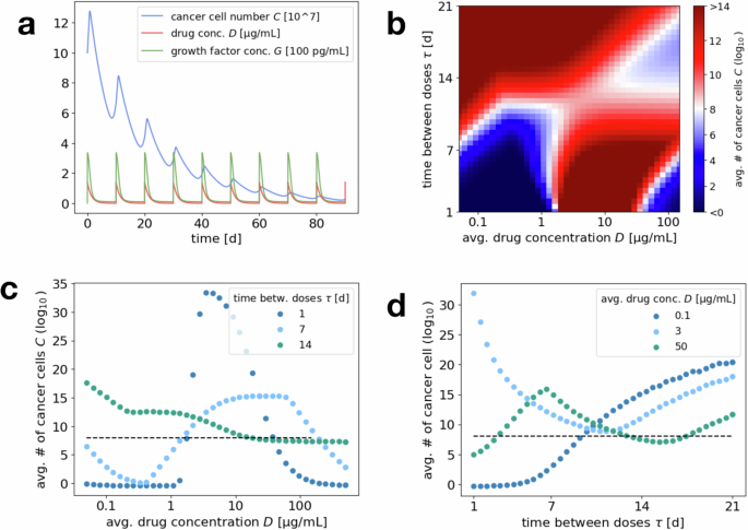
a Example simulation of cancer cell number, drug concentration and growth factor concentration over the course of 90 days for an initial number of 108 cancer cells and an administered drug concentration of 1.4 μg/mL every 10 days. b Heat map of average tumor size over the last 30 days after 180 days of treatment, for varying average drug concentration (x axis) and drug administration schedule (i.e., days τ between administered doses, y axis). Fixing the average drug concentration on the x axis and the time between doses on the y axis automatically fixes the corresponding administered dose. Red regions mark protocols where the cancer cell number increases over time, i.e., failed treatment, while blue regions correspond to protocols that induce a decrease in cancer cells, i.e., more successful treatment. c Horizontal cuts through the heat map, exploring the dependence of the average cancer size on an increasing average drug concentration (and hence increasing administered and total drug dose), for fixed intervals of τ = 1, 7, 14 days between administrations. The dashed line indicates the initial cancer cell number. d Vertical cuts through the heat map, exploring the dependence of the average cancer size on the administration schedule (increasing number of days τ between administrations), for fixed average drug concentrations 0.1, 3, 50 μg/mL. The dashed line indicates the initial cancer cell number.
Note that the cancer cell population undergoes initial positive growth under drug administrations, and later enters a negative growth regime before expanding again at lower drug concentrations. This is due to the fact that we consider parameters for which a nonmonotonic response of the cancer cells to the drug concentration can be observed (see “Drug concentration thresholds for tumor reduction”, and specifically Fig. 2c). Moreover, in accordance with realistic scenarios (like the example in “Application: CRC–CAF interactions”), the dynamics of growth factor secretion and degradation are assumed to be relatively fast compared to the drug decay. We can therefore observe that the growth factor concentration essentially follows the current drug-induced equilibrium concentration (overline{G}(S,D)).
After administration, the drug concentration initially lies above the threshold for triggering a microenvironment response ((hat{D})) but below the critical concentration for negative cancer growth rates corresponding to the maximum growth factor concentration (({D}_{{rm{crit}}}({G}^{max }(S)))). Hence the treatment only becomes effective once the drug concentration drops below (hat{D}) and the growth factor concentration (and with it the critical drug concentration) decline as well. The goal for treatment plan optimization is to maximize the time of the system in the negative growth rate regimen.
Optimal dosing frequency
In order to investigate the effects of varying dosing schedules, we compare regimens in which the average drug concentration in the plasma is conserved, but the frequency of drug administration—and hence the administered dose to achieve this average concentration—are varied. To study long-term success of the treatment, we consider a tumor that initially consists of 108 cells over a total administration period of 180 days (6 months), and protocols varying the time τ between administrations from 1 day to 3 weeks.
For an administered drug concentration of Dadm, we can compute the average drug concentration as
Consequently, to obtain an average drug concentration of Dav through drug administration every τ days, the administered concentration needs to be chosen as
Note that conserving the average drug concentration is slightly different from conserving the total administered drug amount (sum over all administered doses) due to variable decay dynamics between regimens.
To compare the outcome of different dosing schedules, simply comparing the final number of cancer cells after 180 days would not be sufficient. This is because the cancer cell number fluctuates between drug administrations and the final number might hence suggest that a treatment plan is more successful simply because it was sampled during a local minimum. To avoid this effect, we instead compare average cancer cell numbers over the last 30 days (1 month) of treatment, ensuring that at least one entire treatment cycle is covered for all choices of times τ between drug administrations.
Figure 4b displays a heat map plot for the average cancer cell number, varying the average drug concentration and the treatment administration schedule. Figure 4c, d shows horizontal or vertical cuts through this heat map, where either the time between administrations τ or the average drug concentration are kept constant and only the respective other quantity is varied.
From a clinical perspective, both of these viewpoints are interesting to consider. While a frequent administration of drug doses allows the most control over the drug concentration in the plasma, keeping it relatively constant, logistics around treatment administration might dictate a certain schedule of break times τ between drug administrations (i.e., fix a horizontal axis in the heat map plot). Studying Fig. 4c, one can observe that for short breaks (e.g., τ = 1 day), the behavior mirrors the results of “Effective drug concentrations for short-term dynamics”, where both very high and lower concentrations are effective but intermediate concentrations are not (compare Fig. 2). This is because for short breaks administered doses are not too high and the drug concentration does not fluctuate too much between administrations. Intermediate break times (e.g., τ = 7 days) are still similar to shorter breaks in the sense that they show success for both lower and very high administered doses. However, since the fluctuations around the average drug concentration are much larger, the successful windows are narrower. This is because both average concentrations at the upper and lower end of the successful concentration windows yield some time with unsuccessful drug concentrations. For long break times (e.g., τ = 14 days and above), the drug concentration will eventually drop to the intermediate and very low unsuccessful concentration windows either way and hence only very high average (and hence administered) drug concentrations can be efficient by maximizing the time of the successful high concentrations.
Switching perspectives, to avoid drug toxicity and other side effects, there are often restrictions on the admissible average drug concentration, closely related to the total administered drug dose over time. In these cases, it is of interest to find the best drug administration schedule for a fixed average concentration. Figure 4d demonstrates that for low average concentrations (e.g., 0.1 μg/mL, within the window of successful lower concentrations) shorter treatment breaks are most successful. In this case, also the administered drug doses are lower and hence for longer breaks the concentration drops down to unsuccessful low concentrations between administrations. In contrast, for intermediate concentrations (e.g., 3 μg/mL, within the window of unsuccessful intermediate concentrations) slightly longer treatment breaks are advantageous since they allow for the drug concentration to drop down to the lower successful window. Finally, for high concentrations (e.g., 50 μg/mL, within the window of successful high concentrations) both short treatment breaks (that keep the drug concentration in the high successful window) and longer treatment breaks (that let the concentration drop down to the low successful window) can be successful. In all cases, taking too long of a break between administrations eventually becomes unsuccessful since the drug concentration always drops below the lower successful range.
Notably, it is often also necessary to restrict the maximal drug concentration in the plasma, which limits the admissible combinations of average drug concentrations and administration schedules. For example, it is not possible to arbitrarily increase the time between administrations for a fixed average drug concentration, as it increases the administered drug concentration.
The above considerations are summarized in Fig. 5, which shows the drug concentration over time for varying average drug concentrations and treatment administration schedules, switching between successful and unsuccessful concentration windows. Within one plot, one can observe that increasing the time between administrations increases fluctuations around a common average drug concentration. On the other hand, comparing between the three plots, fixing an administration schedule determines the shape of the drug concentration curve and changing the average concentration shifts this curve up or down. The goal of treatment optimization is to—within certain constraints on concentrations and schedules—maximize the overlap of the drug concentration curve with the successful concentration windows.
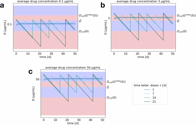
Plots display drug concentration (log10) over time for varying lengths of treatment break (within one plot; 1, 7, 14, or 21 days) and fixed average drug concentrations of a 0.1, b 3, c 50 μg/mL. Blue areas correspond to concentration ranges yielding tumor reduction and red areas to concentration ranges leading to tumor growth, as identified in “Drug concentration thresholds for tumor reduction”.
Application: CRC–CAF interactions
The previous two sections have investigated a general case of cancer treatment response, modulated by stromal cells in the cancer microenvironment. Let us now turn to a specific application and consider the case of colorectal cancer cells (CRC) treated with cetuximab (CTX). CTX is an established anticancer drug that is targeting the cancer cells by blocking the receptor for epidermal growth factor (EGF, EGFR, respectively). This interferes with the cells’ proliferation, inducing a negative tumor growth rate. However, CTX not only impacts the cancer cells but, as experiments have shown, also affects the cells of the microenvironment6. Cancer-associated fibroblasts (CAFs) show increased secretion of EGF when treated with CTX. This increased amount of EGF competes with the CTX molecules for binding to EGFR, hence partially reversing the drug’s effects. As a result, in the presence of CAFs, higher tumor growth rates are observed, making the treatment less efficient.
To parameterize the general model for this specific application, we use data from two sets of in vitro experiments. Monocultures of CRC cells treated with varying concentrations of CTX and EGF allow us to determine the parameters associated to the dose–response curve rC(D, G) by fitting a hill function depending on D to the estimated growth rates for fixed EGF concentrations G. We observe that the slopes k1 of the fitted hill functions do not vary too much and follow no clear pattern, while the value for the inflection point monotonously shifts to higher drug concentrations as the EGF concentration increases. Therefore, we choose a uniform slope and depict the inflection point value as a function D50(G) in G. The parameters for the growth factor concentration (overline{G}(S,D)) are obtained from EGF concentration data from monocultures of different CAF cell lines treated with varying CTX concentrations. We observe a threshold response to increasing drug concentrations that allows us to parametrize a logistic function (overline{G}(S,D)) for the equilibrium EGF concentration. The data shows that a constant maximal growth factor concentration (cf. Eq. (7)), independent of the CAF cell number, best depicts the dynamics of this application. More details of the parametrization procedure are provided in “Methods”.
Short-term dynamics
As a first step, we consider the short-term dynamics of CRC–CAF interactions to identify optimal drug concentrations, using the simplified model of “Effective drug concentrations for short-term dynamics”. We investigate both single-drug treatment with CTX and a combination therapy with EGF-blockers.
Single-drug treatment with CTX: Plugging the parameters from Table 1 into Eq. (4), we obtain that, for a fixed EGF concentration G, the critical drug concentration for therapy success, i.e., the minimal concentration above which a negative cancer growth rate is achieved, is
In particular, this yields that ({D}_{{rm{crit}}}(0)approx 0.71,mu g/mL,>, hat{D}=0.0049,mu g/mL). Thus criterion Eq. (10) fails and the increased EGF secretion by the CAFs is triggered before a negative cancer growth rate (according to the dose–response curve for no EGF) is obtained. We therefore see no nonmonotonic behavior when increasing the CTX concentration, which is supported by Fig. 6a.
a Equilibrium EGF concentration (overline{G}(S,D)), depending on the CTX concentration D (solid line), and critical CTX concentration Dcrit(G), depending on the EGF concentration G (dashed line, axes flipped). Blue lines reflect base parameters, while intensifying orange lines depict increasing effects of EGF-blockers decreasing the maximal (effective) EGF concentration ({G}^{max }). The minimal CTX concentration to induce negative CRC growth rates is determined by the intersection of the solid and dashed lines, i.e., the fixed point concentration D of ({D}_{{rm{crit}}}(overline{G}(S,D))). b Heat map showing the CRC growth rate for varying CTX concentrations D and maximal EGF concentration ({G}^{max }). Red areas correspond to failed treatment, i.e., positive CRC growth rates, blue areas to successful treatment, i.e., negative CRC growth rates. White areas correspond to a sign change in the growth rate and the black horizontal line marks the original original regime.
The (in this case unique) fixed point of (D={D}_{{rm{crit}}}(overline{G}(S,D))), which is the theoretic minimal CTX concentration to induce a negative cancer growth rate, can be calculated as 0.86 μg/mL for the average maximal EGF concentration of ({G}^{max }=27.1) pg/mL and ranges between 0.82 and 0.91 μg/mL for the different patient-derived CAF cell lines studied in the experiments. In this application, since high EGF secretion is triggered at small concentrations of CTX, this fixed point coincides with ({D}_{{rm{crit}}}({G}^{max })). To account for fluctuating CAF numbers, uncertainty in the estimated parameters and to achieve a strictly negative growth rate that causes the CRC cell population to shrink within a reasonable time span, a slightly higher CTX concentration should be chosen in applications.
Combination therapy with EGF-blocker: As briefly mentioned in “Mathematical model” and further discussed in “EGF secretion and varying CAF number/type”, there is no observed correlation between the maximal secreted EGF concentration ({G}^{max }) and the number of CAFs in our specific CRC application. There are slight variations between different CAF cell lines and experimental runs, but in general the secreted EGF levels remain at a stable, relatively low value. Hence, decreasing the number of CAFs does not seem to be a promising approach to increase therapy success.
However, one potential combination candidate class is EGF-blockers (neutralizing antibodies) that can partially neutralize EGF molecules and hence weaken the effects of the microenvironment on the CRC cells (see Fig. 5 in ref. 6). Figure 6 shows the impact of a varied effective equilibrium EGF concentration (e.g., through EGF-blockers). The amount of naturally secreted EGF is generally quite low in comparison to the administered EGF in monoculture CRC experiments, where the most significant shift of the dose–response curve for the CRC growth rate is observed for higher EGF concentrations (cf. “Dose–response curve and D50”). However, particularly for the typical CTX concentration of 1 μg/mL, we can see that a variation of the maximal EGF concentration ({G}^{max }) can make a substantial difference since it is rather close to the critical CTX concentration for negative growth rates under base line parameters.
Since we do not have any nonmonotonic behavior for the CRC–CAF application, blocking EGF has the most impact when combined with a CTX concentration that is close to critical, i.e., the concentration where the cancer growth rate switches sign. As can be seen in Fig. 6b, where increasing the EGF-blocker effect corresponds to shifting down, for lower or higher concentrations, there is not much change in the growth rate. For concentrations around the fixed point of ({D}_{{rm{crit}}}(overline{G}(S,D))=)0.86 μg/mL however, blocking EGF can make the difference by decreasing the cancer growth rate below a threshold that leads to observable tumor shrinking. This effect could become even more relevant under different conditions. For example, if the EGF secretion was higher in vivo, this would increase the range of CTX concentrations for which combination treatment is effective.
The window of CTX concentrations for which combination treatment can lead to an improved therapy outcome is patient specific. As seen in Fig. 6b, it depends on the individual base line maximum EGF concentration ({G}^{max }) (depicted by the black solid line). Hence, for different patients and the same CTX concentration, EGF-blockers might show a much higher effect in some individuals than in others.
Long-term treatment
Having studied the short-term response to certain CTX concentrations and EGF-blockers, we now return to the dynamic model in Eq. (1) to investigate long-term effects of different treatment schedules with breaks between drug administrations. Due to the monotonic drug response in this application, the situation is slightly easier than in “Treatment optimization for long-term outcomes” and we study combination treatment with EGF-blockers (aEGF) in addition to the single-drug treatment with CTX.
Single-drug treatment with CTX: As an initial example, Fig. 7a shows the number of CRC cells and concentration of CTX and EGF over the course of 90 days for a dose of 1 μg/mL CTX administered every 7 days. We see an initial decay of the cancer cell number after every drug administration, which turns to positive growth again once the drug concentration has decreased. Since the drug concentration stays above the threshold value (hat{D}=) 0.0049 μg/mL for increased EGF secretion by the CAFs, the EGF concentration stays constant at its highest possible level of ({G}^{max }=) 27.1 pg/mL.
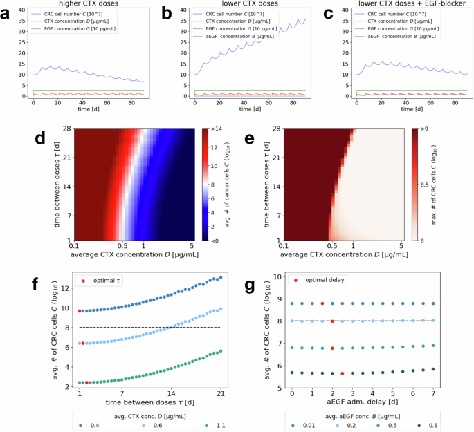
Example simulations of CRC cell number, CTX, EGF and aEGF concentration over the course of 90 days for an initial number of 108 cancer cells and (simulatneous) drug administration every 7 days of a 1 μg/mL CTX, b 0.85 μg/mL CTX, c 0.85 μg/mL CTX and 0.5 μg/mL aEGF. Heat map plots of d average tumor size over the last 30 days and e maximal number of CRC cells for 180 days of treatment, for varying average CTX concentration (x axis) and drug administration schedule (i.e., days τ between administered doses, y axis). Fixing the average CTX concentration on the x axis and the time between doses on the y axis automatically fixes the corresponding administered dose. d Red regions mark protocols where the CRC cell number increases over time, i.e., failed treatment, while blue regions correspond to protocols that induce a decrease in CRC cells, i.e., more successful treatment. f Vertical cuts through the heat map, exploring the dependence of the average CRC cell number on the administration schedule (increasing number of days τ between administrations), for fixed average CTX concentrations 0.4, 0.6, 1.1 μg/mL. The dashed line indicates the initial cancer cell number. Red dots mark the administration schedule that leads to the minimal CRC cell number for the respective CTX concentration. g Average CRC cell number for an administered dose of 0.85 μg/mL CTX every 7 days and varying delay of aEGF administration, for fixed average aEGF concentrations 0.01, 0.2, 0.5, 0.8 μg/mL. The dashed line indicates the initial cancer cell number. Red dots mark the administration delay that leads to the minimal CRC cell number for the respective aEGF concentration.
Due to the relatively slow decay of CTX, there is an initial accumulation of the drug over the course of the first couple of drug administrations and successive treatment breaks, until (fluctuation around) the steady state is reached. As a consequence, one can observe an initial positive net growth of the cancer cell population (averaged over one cycle) before it eventually declines. To evaluate treatment success, one should not only consider the final (averaged) cancer cell number but also take into account the maximal cancer cell number during the entire time of treatment.
Due to drug accumulation, we can observe in Fig. 7d that even average CTX concentrations below the predicted minimal successful concentration of 0.86 μg/mL from “Effective drug concentrations for short-term dynamics” can be successful for short breaks between administrations τ. This is because the average is decreased by the small initial concentration but the higher concentrations later on lead to cancer reduction. Comparing the heat maps in Fig. 7d, e, one can moreover see that for treatment schedules (in terms of average CTX concentration and time τ between administrations) that yield an overall decline in cancer cell numbers (blue areas in (d)), the maximal cell number does also not significantly surpass the initial number of 108 cells. Hence the effect of initial net growth during drug accumulation is not too severe.
Generally, for this application higher CTX concentrations are more successful for all administration schedules. When fixing an average CTX concentration, for example the maximal tolerable amount, we can determine the corresponding optimal time between administrations τ, i.e., the administration schedule that minimizes the final (average) number of CRC cells. Figure 7f shows how this optimal τ increases with the average drug concentration. This can be accredited to the fact that the drug concentration will not decay to the unsuccessful levels as easily for higher doses and slightly longer cycle lengths yield a higher administered dose, which temporarily pushes the system not just to any negative but the lowest growth rate regime. Overall, the optimal τ lies at only few days. However, we see that there is not much variation of the therapy outcome for values of τ between 1 and 10 days, i.e., the optimal administration schedule is not a very strict minimum and one could choose longer treatment breaks to get similar results.
Combination treatment with EGF-blocker: Lastly, we consider a combination treatment of CTX with anti-EGF neutralizing antibodies (aEGF). To this end, we need to extend the mathematical model by an additional component B that tracks the concentration of this EGF-blocker. We prescribe an exponential decay rate dB such that this concentration follows the dynamic
in between administrations. Moreover, we incorporate the effects of EGF-blockers into the cancer cell dynamics by having them (partially) neutralize the effects of EGF. This impact is scaled by a parameter nB and the formula for the D50 drug concentration becomes
EGF-blockers improve treatment success: As can be seen in Fig. 7b, c, adding EGF-blockers to the therapy protocol leads to improved treatment success. For an administered dose of 0.85 μg/mL CTX every 7 days (corresponding to an average concentration of roughly 0.241 μg/mL), which would not be successful by itself, adding aEGF can lead to a positive treatment outcome. This is even the case at an administered dose of 0.5 μg/mL (corresponding to an average concentration of 0.142 μg/mL), which neutralizes less than 15% of the secreted EGF for our parameter choices.
Timing for combination treatment: In Fig. 7c, CTX and aEGF are administered simultaneously. A natural question is to ask whether this is the optimal choice or if an asynchronous administration would be more effective. As can be seen in Fig. 7g, which is an example plot for varying the administration delay for a number of different aEGF doses, the time point of aEGF administration does not seem to have much impact on therapy outcome. This is also supported by a more extensive numerical study for varying base protocols of CTX administration. When looking for the optimal delay, one can observe that a slight delay of 2–3 days seems to be favorable (cf. Fig. 7g). The reason is that directly after CTX administration, its concentration is still high enough to induce a negative cancer cell growth rate by itself. Administering the aEGF with a slight delay, shifts the CTX dose–response curve of the cancer cells at a time when the CTX concentration is already decaying (below a concentration that would be successful without aEGF) and thus extends the time until the cancer cell population starts to expand again. Administering aEGF too late on the other hand would mean that the CTX concentration has already dropped to a level that is ineffective either way.
Notably, even though the effect of a delayed growth factor blocker administration is relatively small in this specific scenario, it might be much larger in cases where it varies the effective EGF concentration around the critical value (hat{G}) (379.4 pg/mL) and not just at an already low level (below 30 pg/mL), which might be the case in vivo.
Discussion
In this paper, we have provided a modeling framework for the interaction of cancer cells and stromal cells in the microenvironment, which allows us to study the stromal impact on therapeutic windows, the impact of combination therapy and the best timing and dosing for long-term treatment with periodic drug administrations and breaks.
As seen in “Drug concentration thresholds for tumor reduction”, as a consequence of different drug concentration thresholds for triggering a response in the cancer cell and stromal cell populations, a non-trivial relation between the drug concentration and the cancer cell growth rate might arise. In particular, the complex interactions between tumor cells and their environment can lead to nonmonotonic drug response profiles, which impact effective therapeutic windows. We demonstrated how these therapeutic windows can be estimated by studying the critical drug concentrations corresponding to different growth factor concentrations. We also investigated how combination with therapies acting via various mechanism (e.g., neutralizing the secreted growth factor or targeting the stromal cells’ drug response) has the potential to manipulate these windows (sections “Combination therapy—targeting stromal cells”, “Combination therapy—targeting stromal drug response”, and “Combination therapy—targeting growth factor efficacy”).
Based on the results of “Effective drug concentrations for short-term dynamics” for constant drug concentrations, we computationally studied the dynamic system of cancer cells growing under varying drug concentrations in a therapy protocol with treatment breaks in “Treatment optimization for long-term outcomes”. We have demonstrated how the specific choice of the treatment schedule (duration of treatment breaks) and the administered drug concentration can optimize treatment success (in terms of minimizing the final cancer cell number) by keeping the drug concentration in the identified successful therapeutic windows for as long as possible. This approach can easily be altered to account for limited feasibility of some treatment protocols. By restricting the range of admissible parameters, constraints such as a minimal time between drug administrations or a maximal overall or temporary drug dose/concentration, which might be necessary to prevent significant side effects, can be integrated.
For our case study of colorectal cancer cell and cancer-associated fibroblast interactions, the relationship between the drug concentration and cancer growth rate is not as complicated (in particular we do not observe non-monotonicity) and there is a single critical threshold above which drug concentrations induce negative cancer growth (see “Short-term dynamics”). Nevertheless, the above framework can be used to optimize therapy outcomes by choosing shorter treatment cycles, to avoid fluctuations of the drug concentration into the lower unsuccessful regime, and administering epidermal growth factor-blockers with a slight delay, to shift the critical threshold down once the drug concentration starts to decrease significantly (as seen in “Long-term treatment”).
Our results suggest that stromal characteristics within a tumor’s microenvironment can impact therapeutic windows and the treatment strategies required to achieve efficacy. However, to translate our approaches to a clinical setting in vivo, further work is necessary. For example, our model would need to be extended to include pharmacokinetic dynamics of the drug distribution. There are additional interaction mechanisms that rely on different molecular (growth) factors and/or the cancer cells themselves inducing a stromal response26. To make quantitative choices about the best treatment strategies, random fluctuations both between individual patients (leading to uncertainty in the system parameters) and of the underlying dynamics (leading to stochastic rather than deterministic behavior) need to be taken into account. As a consequence, aiming for very specific successful strategies (in the sense of hitting narrow successful drug concentration windows) may not be feasible in practice and an additional goal of the optimization process will be to find robust strategies.
As a subject of future work, we would like to study the impact of heterogeneity in the population of stromal cells. Under the current assumption of a non-expanding population of such cells, this is not too relevant, as the stromal cell population enters the equations as a constant and we can simply consider the average dynamics when it comes to the maximum secreted concentration ({G}^{max }(S)). A distinction might however be necessary when the stromal subpopulations show different behavior in triggering a response, i.e., different drug concentration thresholds (hat{D}). In this case, it might be of interest to study dosing regimens that balance effects on cancer cells and triggering only a part of the stromal cell population. Importantly, in systems where the stromal cell population is dynamic or stromal cells are targeted directly, it will be interesting to study the influence of different (e.g., fast expanding or high secreting) stromal subpopulations, particularly when the composition of the stromal cell population is changing over time27. In addition to studying small tumors that are newly emerging or in remission, a heterogeneous stromal cell population could be another scenario in which studying a stochastic (agent-based) Markov process version of the currently deterministic equations might become relevant. If the stromal cell population is composed of smaller subpopulations, random fluctuations may significantly vary this composition and hence influence the resulting cancer growth dynamics. The risk (or promise) of loosing certain subpopulations can be an interesting additional objective of therapy design.
Methods
Parameter estimation
In the following, we describe the parameter estimation for the concrete application of colorectal cancer cells (CRC) and cancer-associated fibroblasts (CAF) interactions under treatment with cetuximab (CTX). Data is taken from experiments of the Mumenthaler lab, partially published in ref. 6. A summary of all parameters for both the CRC–CAF application in “Application: CRC–CAF interactions”, as well as the general model of sections “Effective drug concentrations for short-term dynamics” and “Treatment optimization for long-term outcomes” is provided in Table 1 at the beginning of section “Drug concentration thresholds for tumor reduction”.
Dose–response curve and D
50
As a first step, we determine the dose–response curve of CRC cell growth under varying concentrations of drug (CTX) and growth factors (EGF), i.e., we determine the function rC(D, G). In the specific case of CRC, this is based on monoculture experiments monitoring CRC cell growth under different concentrations of CTX and EGF (see Fig. 8a for the reduced model diagram and Figs. 2, 4 in ref. 6 for the original data).
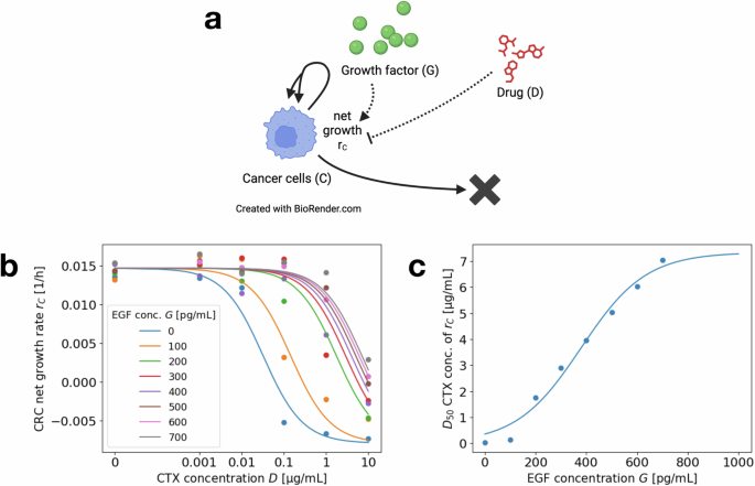
a Interaction diagram summarizing the dynamics of the reduced model for CRC monoculture experiments. Each solid or dashed arrow corresponds to an event that changes the system state. Dotted arrows mark the influence of D and G on the dynamics of C. Created in BioRender https://BioRender.com/o42g88633. b Dose–response curve for CRC net growth rate rC(D, G) depending on the CTX concentration D (x axis), for varying EGF concentration G (different color plots). Single points correspond to experimental data, replotted from ref. 6, curves correspond to fitted functions. Experiments were run for 5 days, with cells seeded on day −1 and CTX and EGF administered on day 0. Images were taken on days 0, 3, and 5 to determine the growth rates. c Inflection point D50(G) of the dose–response curve for varying EGF concentration G. Individual fit results for fixed concentrations as points and fitted function as a curve.
We use this data to fit the dose–response curve
where we choose the parameters ({r}_{C}^{min }), ({r}_{C}^{max }) and k1 uniform across the eight different EGF concentrations and separate values for D50(G). We apply a standard least square fitting method. The results are shown in Fig. 8b. While a fit with varying slopes k1 (depending on the EGF concentration) leads to a slightly better fit for the dose–response curves, there is no clear trend in the dependence of k1 on G. Since the effects of a varying slope on the results in “Effective drug concentrations for short-term dynamics” are minimal, we decide for a uniform choice across varying G to simplify the model.
To parameterize the dependence of the inflection point D50(G) on the EGF concentration, we fit the logistic function
to the values determined by the previous fitting of the dose–response curves. This determines the parameters ({D}_{50}^{max }), (hat{G}) and k2. Again, a standard least square fit is applied. The results are shown in Fig. 8c. As can be seen, there is indeed a saturation effect of the D50-value leveling off eventually for increasing EGF concentrations.
EGF secretion and varying CAF number/type
As a second step, we study the growth factor (EGF) secretion by stromal cells (CAFs). This is based on CAF monoculture experiments monitoring cell growth and EGF secretion of CAFs under varying concentrations of CTX (see Fig. 9a for the reduced model diagram and Figs. 1, 3 and S8 in ref. 6 for most of the original data).
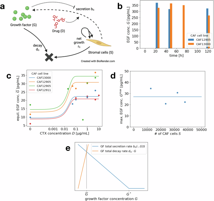
a Interaction diagram summarizing the dynamics of the reduced model for CAF monoculture experiments. Each solid or dashed arrow corresponds to an event that changes the system state. Dotted arrows mark the influence of D and G on the dynamics of S. Created in BioRender32,33. b Experimental data for EGF secretion over time for two different CAF cell lines, replotted from ref. 6. CTX concentration of 1 μg/mL is administered at time 0. c Equilibrium secreted EGF concentration (overline{G}(S,D)) depending on the CTX concentration D, for different CAF cell lines and experimental runs. Points correspond to experimental data, replotted from6, curves to fitted functions. d Maximum secreted EGF concentration ({G}^{max }) for varying CAF cell numbers. Individual fit results for experimental runs as points and mean value as solid line. e Growth factor secretion rate bG(S, D, G) ⋅ S (blue), depending on growth factor concentration G, for fixed number of stromal cells S and drug concentration D. Total growth factor decay rate dG ⋅ G (orange).
Over the course of the experiments (5 days), there was no significant growth of the CAF cell number. As seen in Fig. 9b, the concentration of EGF reaches a high level very fast and stays (almost) stable over the duration of five days. Thus, to model the short-term dynamics, we do not specifically study the rate of EGF secretion but rather assume an equilibrium concentration that depends on the CTX dose and possibly the CAF cell number
We start by fitting the function (overline{G}) for a fixed CAF scenario, i.e., a specific cell line and cell number during one experimental run, with varying administered CTX concentration. To do so, we estimate uniform parameters (hat{D}) and k3 across experiments and individual parameters ({G}^{max }) for the separate experiments. Since the standard least square method overfits for the high data points, we use a slight variation, where the difference between function value and data point are normalized by the function value itself. We thus study the least square fit for the relative error. The resulting curves are shown in Fig. 9c.
To study the dependence of the maximum secreted EGF concentration ({G}^{max }(S)) on the number of CAF cells S, we turn to Fig. 9d. We observe that in this specific case, there does not seem to be a linear dependence but rather a certain low range of EGF concentrations (compared to the up to 700 pg/mL administered in the CRC monoculture experiments) that is obtained independent of the cell number. Hence for the CRC–CAF application we choose the second version of the model from section “Mathematical model”, i.e.,
As the value of ({G}^{max }) we choose the least square mean of the four data points.
Secretion and degradation for treatment with breaks
To determine the parameters for EGF, CTX and anti-EGF (aEGF) degradation, we turn to the literature. CTX has an average half-life of 112 h28, which yields a degradation rate of 0.006 per hour.
EGF has a short circulating half-life of 8 min according to ref. 29, which corresponds to a degradation rate of 5.2 per hour. There generally is a wide range of suggested values in the literature, depending on the specific experimental conditions. For our model, where a fixed equilibrium EGF level is maintained due to the structure of the secretion rate, the dynamics are not sensitive to the exact value of the degradation rate, as long as secretion and degradation occur fast in comparison to the drug decay. Hence we choose a rate of 5 per hour.
In experiments, the impact of EGF is blocked with neutralizing antibodies of IgG type. IgG antibodies have a half-life ranging between 7 and 21 days30, while monoclonal antibodies have a half-life of 11–30 days31. This yields a degradation rate of 0.0009–0.004 per hour, where we consider the worst case (i.e., the fastest degradation) for our simulations.
From the available data, we cannot accurately estimate the secretion rate bG(S, D, G) of EGF. From experiments, we only know that the equilibrium concentration (overline{G}(S,D)) is obtained within at most one day (see Fig. 9b). We model growth factor secretion at rate
where aG is a constant and (⋅)+ denotes the positive part of the difference. The secretion rate bG is hence a decreasing function in the current growth factor concentration G that eventually reaches zero (see Fig. 9e). To balance out degradation at rate dG > 0 and obtain a stable growth factor concentration of (overline{G}(S,D)), G*(S, D) needs to be chosen such that
Note that whether the equilibrium concentration (overline{G}(S,D)) is obtained in praxis depends on the specific scaling of the growth factor secretion and degradation rates. High rates in relation to the drug decay rate make it easier to reach the (drug-dependent) equilibrium growth factor concentration before the drug concentration itself changes too much.
When it comes to choosing parameters aG and G*(S, D), due to the specific form of the secretion rate, a small value of aG automatically gets balanced out by a large G* and vice versa (for fixed equilibrium concentration (overline{G}(S,D))). Simulations confirm that the dynamics are not sensitive to the specific parameter choice and hence we choose aG = 0.001. For a number of 1000 CAFs in our simulations, aGS is therefore of the same order of magnitude as dG and G* is of a similar size than (overline{G}).
Finally, we set the impact of the EGF-blocker as nB = 1. In experiments, a dose of 0.5 μg/mL partially but not fully neutralizes the EGF in CAF-conditioned medium (see Fig. 5 in ref. 6). With our parameter choice, this dose neutralizes half of the present EGF in its impact on shifting the D50 drug concentration.

Responses