Modelling volumetric growth of emerging urban areas around new transit stations

The world is urbanizing rapidly, and developing countries such as India are expected to contribute the most to this urbanization by the year 2050¹. The patterns and trends of urbanization are significantly different for the developing countries. They are primarily location-specific and are often influenced by the heterogeneity of the population. Rapid urbanization would lead to higher productivity, resulting in higher aspirational needs of the urban population. Financial budgeting and the livability of the rising urban population are two critical aspects of coping with these needs². The investment strategies govern the budgeting and the GDP, whereas livability considers the rising demand for urban space. Compact and vertical urban development caters to the higher demand for built-up space while conserving the natural land. The trend of vertical urban expansion has resulted in the transition of urbanization from spatial, i.e. two dimensions to volumetric, i.e. three dimensions. Cities in rapidly urbanizing developing countries are catching up with this trend. Thus, calibrating the volumetric aspect of urban growth becomes inevitable.

Apart from the vertical expansion of the existing urban areas, creating new cities is crucial for catering to the rising urban population in developing countries. The new cities evolve around an infrastructural intervention that can trigger the urbanization process. Transportation infrastructure is one of the most crucial factors triggering the urban growth. The improved accessibility with infrastructure increases the area’s attractiveness for residential, commercial and other purposes^3,4,5. Therefore, capital expenditure in the transportation sector is critical for creating urban areas. Developing countries like India are currently allocating a significant portion of their annual budget to transportation infrastructure development⁶. These investments, especially those in building transit systems, are expected to trigger several new town developments in India. This makes analysing and predicting transit-triggered new town development in developing countries crucial for sustainable urbanization prospects. However, the existing urban growth models are unsuitable for predicting urban areas’ evolution.

Existing literature also lacks the focus on transit-based nodal development in urban growth modelling and prediction, barring a few exceptions^7,8. Most of the past studies focus on predicting the growth of an existing urban area, modelled based on historical trends. Further, all the present urban growth studies worldwide consider only spatial growth. A station developed as a greenfield node is expected to influence the spatial or 2D urban growth significantly^9,10. However, due to land constraints, a brownfield station is expected to influence the area’s volumetric expansion (i.e., spatial and built-up height) through redevelopment plans with increased Floor Space Index^11,12. Previous scientific efforts incorporating the volumetric nature of the cities are limited mainly to observed changes^13,14,15 and do not delve into future predictions. This study demonstrates a model to encapsulate urban growth, focusing on the railway station as a node of urban development. These models predict the spatial evolution of an urban area around the greenfield stations, built far away from the existing cities, and predict volumetric growth of the area around brownfield stations, built at the city’s core.

The existing urban growth models include classical static models of Von Thünen¹⁶, Weber¹⁷, neo-classical models by Lowry¹⁸, Tobler^19,20, and dynamic models such as SLEUTH²¹, California Urban Futures (CUF)²², UrbanSim²³, LandSys²⁴, mainly focusing on only the spatial aspect of urban expansion. A vertical urban growth model is essential for modelling compact cities with sustainable urban growth²⁵. However, the existing modelling methods do not consider the vertical growth aspect and thus cannot predict volumetric urban growth. Moreover, the existing models lack the focus on transit-triggered new town development and primarily focus only on modelling and predicting the horizontal expansion of existing urban areas.

This research fills these three gaps in the existing literature by developing a volumetric urban growth prediction model, considering the heterogeneity and mixed-mode conditions in developing nations. The objectives of this study are (a) to develop a model for transit-triggered urban growth, (b) to predict the volumetric expansion of the existing urban areas, and (c) to predict the spatial evolution of the urban areas around future transit stations. The study also demonstrates the developed models using examples from the potential growth nodes, i.e. future transit stations, in selected cities.

The research flow

This section describes the results of models developed for predicting spatial and volumetric urban growth. The volumetric growth model combines a spatial model for two dimensions (X and Y) and a built-up height model for the third dimension, the dimension of building height (Z). In this article, the spatial growth model is termed a 2D model, whereas the built-up height growth model is termed a D(H) model, representing the height dimension. These two models are developed using historical land cover and built-up height changes. The land cover maps were created through remotely sensed satellite data. The building height data was collected manually through field visits due to the unavailability of digitized building height data²⁵ (For a detailed description of model development, refer to the ‘METHODS’ section). Urbanization trends from a transit-triggered new town in India were thus incorporated through training and validated with the same data. Among many transit infrastructure projects such as urban metro rail in 20+ cities²⁶, suburban and regional rapid rail²⁷, high-speed rail²⁸, etc., only High-Speed Rail (HSR) involves greenfield and brownfield stations.

The greenfield HSR stations, built away from the existing urban areas, are expected to trigger the creation of urban areas around them. Meanwhile, the brownfield HSR stations, which are built well inside the city, are expected to trigger vertical expansion of the existing urban area around them. The upcoming Mumbai-Ahmedabad HSR corridor in India satisfies all the requirements and assumptions of the developed models. Moreover, the Mumbai – Ahmedabad region falls in the same socio-spatio-economic strata as that of Mumbai – Navi Mumbai region in the past. Thus, the developed models were applied to upcoming High Speed Rail stations in India. This section consists of three model development steps – Training, validation, and application of the model. The flow of this section is described in Fig. 1.

Research Flow.

Full size image

Selection of sites

Both greenfield and Brownfield sites were considered for model training and model application purposes. The model was trained with data from Navi Mumbai and Vashi, whereas the model was applied to seven HSR stations of the Mumbai Ahmedabad HSR corridor. Figure 2 shows the sites selected for model training and model application purposes.

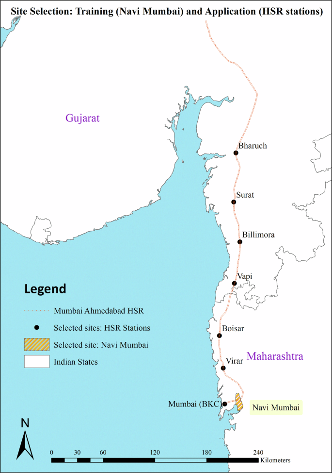
(Sources: HSR station locations from feasibility study report³² and Training data location from literature^29,30,66).

Full size image

Navi Mumbai is a new town developed to decongest Mumbai²⁹ (see Supplementary Note 1 for the locational details). Navi Mumbai consists of 14 development nodes located along a central transit corridor³⁰. This transit corridor (known as the harbour line) was established gradually from 1992 till 2004³¹. The urban growth of Navi Mumbai matches the period of transit development, which is evident from the time-series land cover maps (see Supplementary Note 2 for historical land cover maps). Hence, the 2D model was trained using land cover maps of Navi Mumbai from 1988 to 2008 to match the development timeline of building transit stations in the study area.

Among the 14 nodes of Navi Mumbai, Vashi is the most developed and “sought after” node³⁰ with most commercial developments, malls and high-rise residential buildings. Vashi has the first and the oldest transit station in Navi Mumbai, opened in 1992³¹. Hence, the Vashi station area was chosen to train the D(H) model. This model was trained using building height change data from the same time frame as the 2D model, i.e. 1988 to 2008. The changes in the Vashi station area buildings’ heights from the same period are shown in Supplementary Note 2.

India’s first High Speed Rail corridor is under construction (as of 2022) between Mumbai and Ahmedabad³². This HSR corridor connects important cities of India like Mumbai, Ahmedabad, Surat, and Vadodara²⁸ (see Supplementary Note 1 for locations). Table 1 shows the list of all Mumbai – Ahmedabad HSR corridor stations, the type of development, and the description of their locations.

Seven of these twelve HSR stations were chosen for applying the model to predict the built-up volume. The Mumbai (BKC) station was considered a brownfield station development case, whereas Virar, Boisar, Vapi, Billimora, Surat, and Bharuch were taken as six greenfield cases.

Model outline

Two models were developed for predicting spatial or 2D growth and building height or D(H) growth. The 2D model was developed using the land cover maps of Navi Mumbai from the year 1988 till the year 2008 at an interval of 5 years, whereas the D(H) model was developed using building height maps from the same years with the same interval. The 2D model determines one out of four land cover classes³³ – waterbodies, green cover, barren/open, and built-up with the help of self-transition potential, neighbourhood characteristics, proximity to the transport network and topography³⁴. The D(H) model predicts the built-up height as low-rise, mid-rise and high-rise¹⁵ using the neighbourhood characteristics and transport network proximity (For the details on variables in the model, kindly refer to the ‘Methods’ section). The data from 1988 to 2003 was used for model training, and the 2008 data was used for validation. The model uses the Logistic Regression-based Cellular Automata technique for calibration (Details in the ‘Methods’ section). The following sub-section elaborates on the results of both the calibrated models.

Model results

The parametric coefficients of factors affecting land cover change are given in Table 2. The four vertical columns represent the parametric values for the transition of the central cell to the corresponding four land cover classes. The rows represent urban growth factors and their effects on transitioning the central cell to four land cover classes. These factors and corresponding variables are detailed in the ‘Methods’ section.

The self-transition potentials were the highest for the same land cover classes, indicating the inertia of cells against changing themselves to a new state. In the absence of all other factors, a cell is likely to remain in the same land cover class as it was at the beginning of the simulation. However, the self-transition coefficient of barren to built-up was higher than other classes, indicating that a cell can self-transform from barren to built-up in certain favourable cases. The neighbourhood effect of every land cover class was highest for the same land cover class, showing the nature of the land cover class in converting the central cell to that class. The central cell of a Moore neighbourhood thus changes to the most abundant land cover type in the neighbourhood, creating the homogeneous clusters of land cover classes. However, the cells with multiple major roads in the neighbourhood are more likely to convert to barren/open cells.

The effect of proximity to transit stations is positive for built-up growth. Cells closest to the railway stations are most potent for converting to built-up land. As the distance from the station increases, the coefficient for built-up land cover decreases monotonously, showing the decreasing potential of land cells away from the railway station. In the case of roads, this trend is not monotonous. However, the built-up land class coefficient is the highest for cells less than 0.25 km from the road. Among the topographic variables, the slope shows that cells on flatter terrain are much more likely to convert to built-up than on steeper terrain. Moreover, cells with higher elevation from the mean sea level are mostly green covers and barren/open lands, i.e. forests and hills. The model also incorporates the policy decisions taken to protect hill slopes and green cover on hills through these variables.

The model was validated using the 2008 land cover map of Navi Mumbai. The model accuracy is 83.88%, and the Kappa coefficient is 0.76. The F1 scores of waterbodies, green cover, barren/open, and built-up classes were 0.95, 0.77, 0.76, and 0.82, respectively (See Supplementary Note 3 for the prediction-success table). Figure 3 shows the predicted and actual land cover maps of Navi Mumbai from 2008. These maps were used for model validation. The visible difference in both the maps (contributing to 16.12% of the model’s inaccuracy) is due to the densification of built-up area³⁵ arising from the neighbourhood effects in the Cellular Automata model, as observed above.

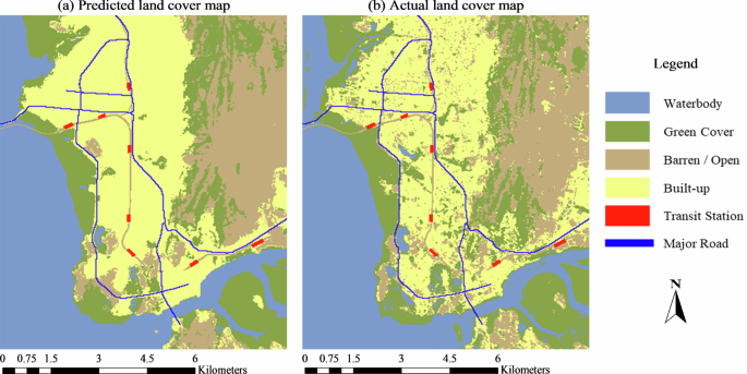
Validation Maps for 2D model – Navi Mumbai 2008.

Full size image

The built-up land class predicted in the 2D model was divided into three classes according to the built-up height for the D(H) model. The three classes were low-rise (height ≤ 9 m), mid-rise (9 m < height ≤ 30 m), and high-rise (height > 30 m)¹⁵. The parametric coefficients for factors determining these building height classes are given in Table 3. The three vertical columns represent the values corresponding to three building height classes, whereas rows represent the factors and magnitudes of their effects.

The neighbourhood effect of the three building height classes was the highest for the same building height class, indicating that any built-up cell will get converted to the building height class most abundant in its vicinity. In other words, a high-rise promotes a high-rise nearby, a low-rise promotes a low-rise, and a mid-rise promotes a mid-rise in the vicinity. The neighbourhood weightage of the built-up area was highest for conversion to the low-rise building, signifying that densely built land parcels are likely to be low-rise. Dense low-rise development in urban set-ups indicates slums worldwide³⁶ and in India^37,38. The neighbourhood effect of the road was highest for conversion to mid-rise built-up land, showing that a higher density of roads promotes mid-rise growth in the vicinity.

The distance from the railway station had the highest coefficients for the mid and high-rise built-up areas. Land cells closest to the railway station, i.e. located within a 0.25 km radius from the station, had the highest weightage for converting to the mid-rise built-up land. Subsequently, land cells between 0.25 to 0.5 km from the railway station had the highest weightage for mid-rise, followed by high-rise. The cells located farthest from the railway station (beyond 1 km) had the highest propensity to convert to low-rise built-up land. On the contrary, cells closest to the road (i.e. within 0.125 km) were most likely to get converted to the low-rise built-up land. The cells farther from the road had a higher propensity of conversion to mid-rise, followed by low-rise. The weights of proximity parameters show the effects of transport infrastructural development in vertical urban growth.

Similar to model 1, this model was validated using Vashi’s 2008 building height map. The model accuracy was 83.73%, with a Kappa coefficient of 0.90. The F1 scores of low-rise, mid-rise, and high-rise classes were 0.91, 0.85, and 0.62, respectively (See Supplementary Note 3 for the prediction-success table). Figure 4 shows Vashi’s predicted and actual built-up height maps for 2008.

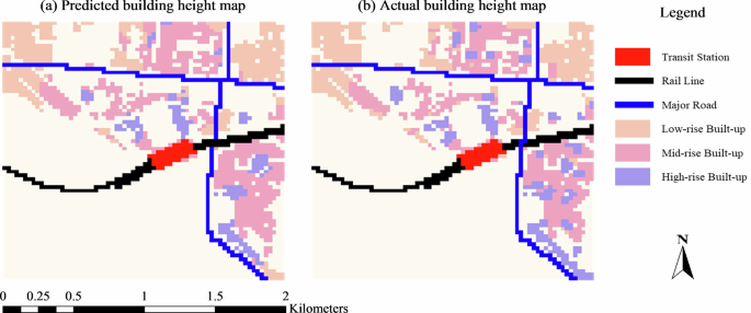
Validation Maps for D(H) model – Vashi 2008.

Full size image

The two developed models were applied to the station areas of upcoming HSR stations in India to predict the built-up volume change around these stations in the next 20 years.

Model application

HSR stations from India’s first upcoming corridor consist of greenfield and brownfield stations (see Table 1). The greenfield stations induce the development of built-up areas, promoting spatial (2D) expansion. On the other hand, brownfield stations impact the vertical expansion of existing built-up areas around them, resulting in 3D urban growth. Thus, the urban growth around greenfield HSR stations was predicted using only the 2D model, whereas the combination of 2D and D(H) models was used for brownfield stations. The emergence of an urban area in 2D and the expansion of an existing urban area in 3D were predicted for seven HSR stations. The simulations were conducted for the next 20 years, with a 5-year interval between two consecutive predictions (see Supplementary Note 4 for all prediction results). Two examples of these predictions are provided in this section.

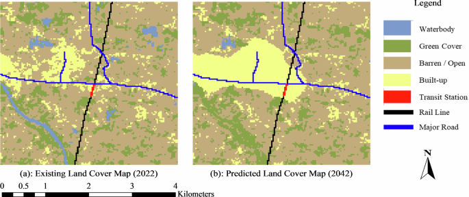
Figure 5 shows the existing and predicted land cover, built-up heights and 3D building maps of the Mumbai (BKC) HSR station area. An area of 4 sq. km centred around the future HSR station of Mumbai (BKC) was considered for model application to determine the volumetric urban growth over the next 20 years. The existing maps are from the year 2022, whereas the predicted maps are for the year 2042.

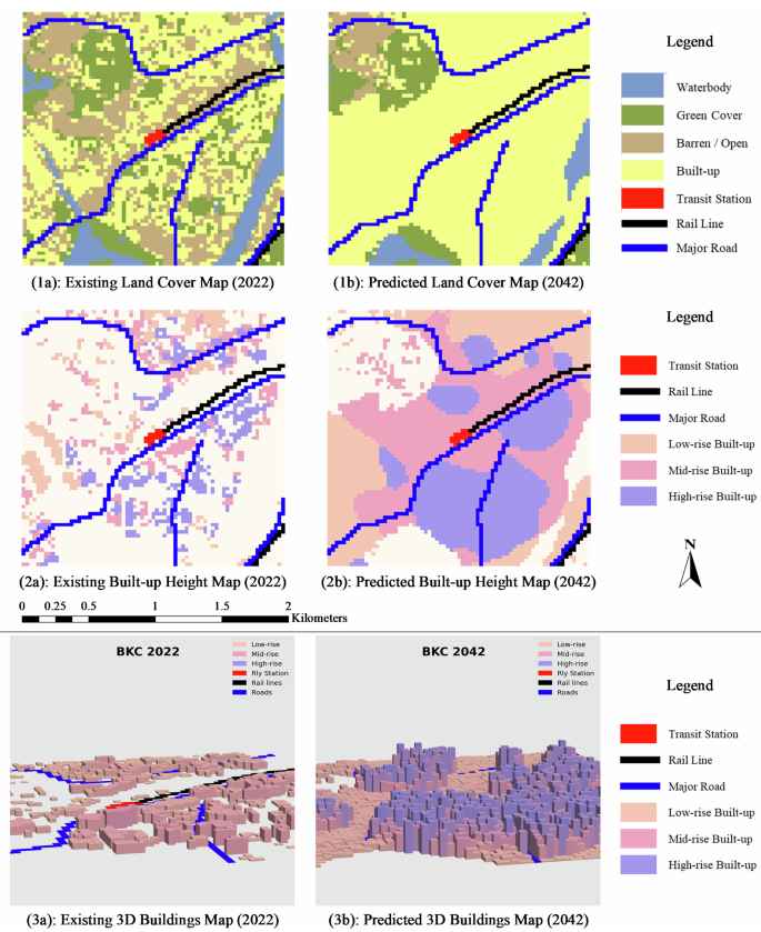
Model Application – Brownfield station (Case of Mumbai BKC).

Full size image

Figure 5(1b) depicts the significant growth of the built-up area around the upcoming HSR station in Mumbai (BKC) in the next 20 years. Figure 5(2b) highlights the rapid growth and clustering of high-rise built-up areas closer to the HSR station and road.

Similar to Mumbai (BKC), an example of Billimora Greenfield HSR station’s area development is illustrated in Fig. 6. An area of 16 sq. km. around the upcoming greenfield HSR stations was considered for model application. The 2D model predicts that Billimora HSR station will promote large-scale built-up development. The simulation results show that the new town developed around the HSR station would grow and merge with the existing town on the West side of the station.

Model Application – Greenfield station (Case of Billimora).

Full size image

The detailed simulation results of all six greenfield stations and one brownfield station have been described in Supplementary Note 4. The results include the land cover and building height predictions at every five-year interval from 2022 to 2042, i.e., the next 20 years.

This research develops a three-dimensional urban growth prediction model for transit-triggered urban development in developing countries. The developed model attempts to fill three gaps in the existing literature – (1) Non-consideration of building height change in the prediction, (2) Inability to predict newtown evolution, and (3) Lack of transit infrastructure triggered urban growth models. The model is developed using a cellular automata-based multinomial logistic regression approach (The modelling details are explained in the ‘METHODS’ section). The spatial evolution and built-up height growth models were trained and calibrated using the urban growth patterns of Navi Mumbai – a new town in India developed around the central transit corridor³⁰. The developed models were then applied to the future greenfield and brownfield transit developments in India – stations of the first High Speed Rail corridor in India between Mumbai and Ahmedabad, to predict future urban growth. The volumetric urban growth was predicted for the existing urban areas around the brownfield HSR station, whereas spatial evolution of a new town area was predicted for the greenfield HSR station. The advantages and shortcomings of the developed models are discussed in this section.

The restrictions on building height are often relaxed in the future to avoid excess spatial expansion and provide welfare gains^12,39. These relaxations increase the Floor Area Ratio, adding more built-up area vertically. This unplanned vertical growth increases the stress on services and infrastructure^40,41, creates congestion⁴², and decreases the Quality of Life⁴³. Our model overcomes these gaps by considering the built-up height in urban growth prediction. The developed volumetric urban evolution model would help in planning better cities. This volumetric urban growth study can contribute to modelling compact and sustainable cities²⁵ with optimal size and occupancy⁴⁴, maintaining a standard quality of life⁴⁵.

Nevertheless, the lack of large-scale historical building height data mandated the primary data collection on existing and historic building heights for modelling purposes. This significantly reduces the influence area around brownfield HSR stations that can be considered for built-up height growth. The significant variations among building heights could be captured better with a continuous model of built-up height instead of a discrete model with low, mid and high-rise choices. However, the smaller data size restricts continuous models’ usage. Lastly, the unavailability of the history of government regulations, floor space index distribution, and other policies restrict the model from considering only the infrastructural or built-environment aspect.

Transit Oriented Development (TOD)¹¹ is among the most researched transportation and urban planning topics. However, the research and the Indian government’s norms on TOD⁴⁶ restrict themselves to only urban transit systems, such as the metro. The on-ground implications of TOD policies must be studied through ex-post studies of such locations, especially in underdeveloped and developing countries. Analyzing the urbanization patterns of a city developed with TOD principles can help build models that can predict TOD-based new town development. The existing urban growth models use the historical development of existing cities to predict the future growth of the same cities. Thus, these models are incapable of predicting a new town development trajectory. This research attempts to develop a model that can predict emergence of an urban area around a transit node. The developed models can help in systematic planning of transit-oriented development in developing countries.

The developed models predict horizontal and vertical urban growth, considering only the built-environment intervention, i.e., transit stations, as the primary trigger. Land’s financials and market dynamics are primarily location-specific and reflect their effects on the observed urban growth. Thus, among all the external factors, the developed model considers only transportation factors explicit, whereas all other factors, such as financial aspects and policy interventions, are assumed to be implicit. This allows the models to be transferred and applied to any location with a similar socio-spatial-economic background, expecting a future transit development. Moreover, historical land change patterns are unavailable for a new town development around a greenfield station. Thus, models trained at different yet socioeconomically similar locations must be applied. To avoid locational specificity and ensure transferability, the developed model limits itself to only built environment considerations (transit stations and roads) as external factors, along with the internal factors of self-transition, topography and neighbourhood effects.

The developed models were applied to future transit stations in India considering the Business As Usual (BUA) scenario. The BUA condition provides predicted land cover and building height maps for the next 20 years, considering no new infrastructural or policy intervention is made apart from constructing a transit station. The simulation results provide crucial insights for planners, practitioners, researchers and policymakers. A few critical insights are as follows:

1. (a)

   All land cover classes and all built-up height classes push for the neighbouring cell to convert to the same class, thereby promoting cluster formation. This phenomenon replicates and predicts the extensive patch-based development of slums, middle-income housing, and high-rise complexes.

2. (b)

   The development of transit stations alone cannot promote high-rise development in the station area. Transit development, when supported by highway connections, encourages high-rise growth.

3. (c)

   High and mid-rise building growth stagnates over time as the spatial densification of built-up land leads to more low-rise development.

4. (d)

   The urban development around the greenfield transit station is higher when supported by a close connection with an existing urban area.

Apart from the BUA scenario, the models can simulate the scenarios with policy interventions such as development control regulations restricting building heights and ecological zoning restricting built-up development. The models are robust enough to consider infrastructural interventions, such as new road construction, and produce the corresponding prediction results during the simulation years.

The models demonstrated in this paper use the cell size of 30 m*30 m, which is restricted by the resolution of the available satellite data. However, the modelling framework can adopt any cell size, provided such data is available. The availability of extensive building height data can significantly improve the model’s accuracy and predictability under the same framework. Additionally, the models can be improved further by incorporating the variables for accessibility changes, transit ridership data, and residential and commercial location choice submodels. Nevertheless, the developed models’ prediction capabilities are highly suitable for futuristic planning considering the urban density⁴⁷ for optimizing public service utilization⁴⁸.

Our study aimed to create a model for predicting the transit-triggered emergence of an urban area and volumetric urban growth. The urban growth patterns were derived from the historical land cover and built-up height changes of Navi Mumbai and its most developed node – Vashi. This section provides details of the data and the models’ design. Figure 7 describes the methodological flow of this study.

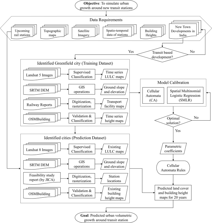
Methodological Flow Diagram.

Full size image

Data

Remotely sensed earth images from LANDSAT with 30 m resolution are the most widely used satellite imageries in the literature^33,49,50,51. These satellite images acquired from the United States Geological Survey’s (USGS) website were used to generate land cover maps using supervised maximum likelihood classification⁵². The historic satellite imageries generated temporary equidistant land cover, terrain, and transportation maps of the city over 25 years. Recent studies on land cover modelling have used four to five classes of land cover³³. The 30 m*30 m land cells were classified into four classes: waterbodies, green cover, barren or open land, and built-up areas. The land cover class waterbodies included oceans, rivers, lakes, artificial reservoirs, and wetlands. Green cover included forests, fields, parks, sanctuaries, and mangroves. Inhabited, non-agricultural, and open land parcels were included in the barren land class. The built-up area consisted of residential, commercial, and industrial buildings and services infrastructure. The classified land cover maps were verified and validated through field checks and with the help of Google Earth images.

The slope of land and elevations from the mean sea level for the desired area of the city were calculated using the SRTM DEM maps acquired from the USGS website. The network of major roads in the city was digitized with the help of the OpenStreetMaps (OSM) base layer, and their temporal evolution was traced using satellite images of each time step. The railway stations were located and digitized using OSM and satellite imagery, and their construction timeline was acquired from the historical development data of Indian railways³¹. Buffer zones of 0.25 km, 0.5 km, 1 km, and 2 km from the major roads and railway stations were drawn. The distances were chosen based on the National Transit Oriented Development Policy of the Government of India⁴⁶ and the future HSR station development plans proposed by the Japanese International Cooperation Agency (JICA)³². These buffer zones were used to calculate transport proximity variables. The building height data of the study area was gathered through field data collection. The building heights were classified into three classes, viz. low rise (less than 9 m), mid-rise (9 to 30 m), and high rise (above 30 m)¹⁵, excluding the areas with no built-up. All the vector layers were rasterized to 30 m*30 m cell size to match the cell sizes of other participating raster layers, i.e., land cover maps and elevation maps.

Modelling

The prepared data was used to train and calibrate the Spatial Multinomial Logistic Regression (SMLR)⁵³ based Cellular Automata (CA)^25,52 model. The Logistic Regression coupled CA is widely used in the literature for modelling spatial growth⁵⁴ and the 3D growth in quasi-form¹⁴. To ensure proper integration of input GIS raster files with the CA environment, the cell in CA must resemble a raster cell⁵⁵. Due to the unavailability of historical satellite data with a resolution finer than 30 m, all raster datasets and the CA models have square-shaped cells with sizes 30m^33,35. A cell can have four states corresponding to four different land cover types. A cell in the land cover state ‘built-up’ can have three states of built-up heights. Moore neighbourhood of size 15 cell * 15 cell was defined around the central cell. This neighbourhood size was found to be most suitable through an iterative process. Thus, the neighbourhood effect is confined to 224 cells in a square grid around the cell for changing its state. The neighbourhood type and size were decided after rigorous trials of various sizes based on the highest modelling accuracy. Many studies on CA-based modelling consider the time step for transition to be 10 years^50,51,56.

However, for a rapidly urbanizing country like India^57,58, a shorter transition time in urban growth modelling can lead to more accurate results³³. The CA-SMLR model developed in this study considers the time step of transition to be five years, similar to the recent studies of other Indian cities³³. The Cellular Automata rules for land cover and building height transition were defined by calibrating the CA-SMLR model with the training data of an identified Indian city with a transit-dependent growth pattern. The CA-SMLR model was calibrated by identifying the transition probabilities of change in land cover and built-up height class.

The probability of transition of a land cell (X, Y) to a land-cover type ‘(i)’ for a given land cell was defined as per Eq. 1

Where,

Where (alpha) is the constant, Self Transition and Neighbourhood effects are specific to land cover class (i), whereas Proximity and Topography are specific to the cell (X, Y).

Similarly, the probability of transition to a building height type ‘(i)’ for a given built-up cell was defined as per Eq. 2.

Where,

Where (beta) is the constant, the Neighbourhood effect is specific to the built-up height class (i), and Proximity is specific to the cell (X, Y). The utility of any land cover or built-up height class was defined as the linear combination of the corresponding influencing factors and a constant. The formulation of these factors is explained here. The self-transition potential was defined as shown in Eq. 3

Where,

The neighbourhood effect was defined as the weighted sum of the proportion of four classes in the neighbourhood. The formulation for the same is as per Eq. 4.

Where,

The proximity factor addressed the cell’s proximity to the transport network. The proximity to transportation facilities was a direct distance to the nearest road cell or transit station. The distance was calculated as Euclidian due to the unavailability of a detailed historical road network. The distance from major roads and distance from railway stations were segregated into five categories with four dummy variables each. The categories were as follows:

1. 1.

   Distance from the major road

   1. a.

      (0,{km}le {distance}le 0.125,{km})

   2. b.

      (0.125,{km}, <, {distance}le 0.25,{km})

   3. c.

      (0.25,{km}, <, {distance}le 0.5,{km})

   4. d.

      (0.5,{km}, <, {distance}le 1,{km})

2. 2.

   Distance from the nearest railway station

   1. a.

      (0,{km}le {distance}le 0.25,{km})

   2. b.

      (0.25,{km}, <, {distance}le 0.5,{km})

   3. c.

      (0.5,{km}, <, {distance}le 1,{km})

   4. d.

      (1,{km}, <, {distance}le 2,{km})

The topography factor included slope and elevation as two variables. The DEM maps were used directly as elevation variables with the cell’s elevation above the mean sea level in hundreds of metres. The slope data calculated from DEMs was converted into a binary variable with

It was assumed that an existing built-up cell, at any stage in the simulation, would not change back to other classes during the simulation period⁵⁹.

Optimization

The model was calibrated in Python with the ‘scikit-learn’ library for logistic regression^60,61,62. This approach allows the integration of machine learning models and their computational power with traditional statistical modelling techniques, such as multinomial logistic regression. Though the land cover classes (4) and built-up height classes (3) were non-binary, the classes are neither ordered nor dependent on each other. Thus, the choice of each class is a binary choice, independent of other classes. Therefore, the One-Over-Other or ‘ovr’ method was used for multi-class classification. The negative log-likelihood function for a given land cover or building height class was thus set in its binary format, as shown in Eq. 5.

Where,

(Pleft({y}_{i}=1left|{X}_{i}right.right)=frac{1}{1,+,{e}^{{-U}_{{land; cover; or; built}-{up; height; class}}}}) is the probability of class being the given land cover or built-up height class for instance i. Thus, the objective function is defined as per Eq. 6.

The above function is optimized to calculate the coefficients of all X values in the utility equation ({U}_{{given; class}}). Considering the non-linear nature of the log likelihood function in the logistic regression, quasi-newton methods⁶³ are best suited for minimization of the function. The standard Broyden–Fletcher–Goldfarb–Shanno (BFGS) algorithm is among the most widely used and best-performing quasi-newton optimization method⁶⁴. Among all the variations of modern quasi-newton optimization methods, the limited memory variant has been observed to outperform all others⁶⁵. Thus, the optimization algorithm used for this study was the ‘Limited memory Broyden–Fletcher–Goldfarb–Shanno’ or ‘lbfgs’ algorithm^61,62. The L-BFGS algorithm requires a doubly differentiable continuous function. Thus, the penalty or loss function considered for the optimization process was the sum of squares of residuals or ‘l2’. The quasi-newton algorithms use the iterative approach. The maximum number of iterations for this optimization was set to 10,000, one of the most commonly used limit⁶¹. The parametric coefficients of contributing variables were used to define the CA rules for land cover and building height transition.