Multi-century geological data thins the tail of observationally based extreme sea level return period curves

Introduction
Extreme tropical and extratropical cyclones produce storm surges that, together with astronomical tides and relative sea-level rise, can cause devastating flooding in coastal communities1,2,3. Local decision-makers employ estimates of return periods for extreme water levels to help plan for future events4. As uncertainties in future storm surges and relative sea-level rise can drastically alter projections of potential damages to the coast5, having precise estimates of return periods is ideal for accurate risk assessments and prudent planning6.
Observationally driven estimates of the return periods of extreme water levels have previously been generated by applying frequency analysis to tide gauge records using extreme value statistical theory7. In this analysis, a parametric family of probability distributions is assumed to describe a subset of the more extreme observed water levels (e.g., the highest water levels recorded by a tide gauge). The probability distribution is then extrapolated to determine the water level at any frequency, even for those most extreme events that are too rare to be captured regularly via observations8. Typically, one of two approaches is used for this analysis9: (1) a block maxima approach, where only the maximum water levels in a given time block (e.g., one year) are evaluated using a Generalized Extreme Value distribution (GEV)8,10,11; or (2) a peak-over-threshold (POT) approach, in which all values over a chosen threshold are evaluated using a Generalized Pareto distribution (GPD)1,4,12. Studies have demonstrated the benefits of using a POT approach given the additional data available for analysis over using a block maxima approach, which generally limits datasets to a single observation a year13,14,15.
Point process models are used to characterize random point occurrences, typically along a time axis, such as the occurrence of an extreme water-level event16. One-dimensional Poisson Point Processes are the canonical point process model7,16. These models become two-dimensional (2D) when a value is associated with the occurrence, such as the occurrence of an extreme water-level event of a specific height16,17. Therefore, following this example, a 2D Poisson Point Process can be used to model the occurrence of extreme water levels, while a GEV or GPD models the extreme water-levels’ magnitudes (over a given threshold for GPD)17. The probability of annual exceedances of extreme water levels have been estimated with GEV and GPD models fitted with tide gauge data and synthetic data1,18,19.
Issues arise when using short observational records to characterize the rarest, extreme events. While tide gauges produce records with little uncertainty in water level or time, they offer a limited sample of extreme water-level events, making it difficult to capture changes in long-term frequency patterns1,6,20. Additionally, having few observations of extreme water levels can lead to large uncertainties in the return levels of low-frequency events7. One way to reduce this uncertainty is to increase the number of extreme observations in the dataset being evaluated. Increasing the number of extreme water-level observations beyond the tide gauge record can be accomplished by using: (1) surges from synthetic storms1,3,21,22; (2) historical accounts and records of storm surges6,15,23; and (3) geologic storm records.
Historical records were first utilized in the field of hydrology and were shown to improve estimates of extreme flood frequency over using instrumental records alone24,25. These findings were late expanded to coastal settings where historical data were shown to improve frequency estimates of extreme surges and water levels15,23. While historical data have proved beneficial, there are still longer-scale records locked in geologic archives that could further constrain estimates of extreme water-level return periods.
Geologic records of extreme water-level events are typically found in the form of allochthonous sedimentary material in back-barrier environments that have been transported via a storm surge from offshore26,27,28. These deposits only capture the most extreme water-level events of the past several thousands of years29. They provide no information on the climatology of the responsible storm (e.g., track, size, proximity, intensity) or water-level height29. The ages of pre-historic deposits are determined indirectly via radiocarbon dating of organic material above and below each deposit26,30,31,32,33. Hence, geologic records of extreme water-level events provide no water height data and temporal data with some degree of uncertainty; they are only indicative that an extreme water-level event has taken place at some time in the past. Therefore, while geological data extend the record of extreme water levels, they do not have the resolution or precision of tide gauge records.
Here, we investigate how the inclusion of geologic records of extreme water-level events in return period calculations affects the uncertainty levels of those estimates in a POT framework. We construct a 2D Poisson point process model that uses tide gauge and geologic data independently to calculate the expected number of events from extreme water levels. Model parameters are estimated via Bayesian optimization and calculated Bayesian credible intervals for the expected number of annual events for every water level based on the modeled parameter estimates. We contrast the return period estimates calculated from tide gauge data alone with those calculated from a fusion of tide gauge and geologic data. We first test the method using synthetic data, then apply the method to two case studies: (1) using tide gauge data from the Woods Hole, MA, tide gauge and a published geologic record of 31 paleo-extreme water levels from Mattapoisett Marsh, MA28,34; and (2) using tide gauge data from the The Battery, NY, tide gauge and a geologic record of 8 paleo-extreme water levels from Cheesequake State Park, NJ35 (Fig. 1).

Site map showing location of data used in the two case studies: (1) Mattapoisett Marsh geologic record (Boldt et al.28, Castagno et al.34) and Woods Hole tide gauge and (2) Cheesequake State Park, NJ (Joyse et al. 35) and the Battery tide gauge.
Results
Synthetic Data
Synthetic data were sampled from a Student’s t-distribution, the parameters of which were chosen to fit de-trended daily maximum data from the Battery, New York City tide gauge (https://tidesandcurrents.noaa.gov/datums.html?id=8518750). Daily maximum water level records were sampled over a 1000-year period. An observable tide gauge record was created from the last 80-years of the 1000-year record, and a geologic record was created using the timing of water-level observations exceeding a 1.35 m threshold over the 1000-year time period. A series of 1000 sets of synthetic data were generated for parameter estimation and model validation (see Methods for further details).
Including geologic data, compared to using the observational tide gauge data alone, significantly decreased the uncertainty in return period estimates for extreme water levels for a random single set of synthetic data (Fig. 2). For example, the width of the 90% credible (5th–95th percentile) range for a 1-in-100 year return period water level (a water level with a 1% chance of annual exceedance) decreased by 47% with the addition of geological data. For a more extreme 1-in-1000 year water level (a water level with a 0.1% chance of annual exceedance), the width of the 90% credible return period interval decreased by 53% with the addition of geological data.
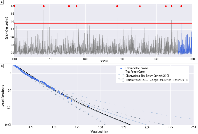
A Gray curve shows the detrended daily maximum water levels from the unobservable 1000-year tide gauge record over the 99th percentile threshold emplaced for tide gauge data. The corresponding truncated 80-year tide gauge record is overlayed in blue, and red dots represent extreme water levels that would be captured in the geologic record given the geologic threshold of 1.35 m. B Empirical exceedances above the 99th percentile (0.56 m) of all tide gauge data shown for the 80-year tide gauge record in blue. The true exceedance curve calculated from the Student’s t-distribution from which the data is generated is in black. The light blue curves show the 50th percentile estimates with the 90% credible intervals for the expected number of exceedances per year calculated from model results using the 80-year tide gauge data alone. The dark blue curves show the 50th percentile estimates with the 90% credible intervals for the expected number of exceedances per year calculated from model results using the 80-year tide gauge and geologic data.
For a random single set of synthetic data, median estimates of water levels with a 10%, 1%, and 0.1% chance of annual exceedance were lower when geologic data were included (Fig. 2, Table 1). Median estimates of water levels with a 10% and 1% chance of annual exceedance were similarly close to true values (1.02 and 1.40 m, respectively) when geologic data were included (1.00 and 1.37 m, respectively) versus when tide gauge data alone were used (1.02 and 1.44 m, respectively). However, for a water level with a 0.1% chance of annual exceedance, median model estimates when geologic data were included (1.82 m) were closer to the true value (1.83 m) compared to when tide gauge data alone were used in model estimates (2.00 m).
The reductions in uncertainty provided by the addition of geological data are reflected in the estimates of the parameters of the statistical model, which narrow as geological data is added to the tide gauge data (Supplemental Table 1). Model estimates for the geologic threshold (tau) were 1.36 ± 0.07 m, while the true value used to generate the synthetic geologic data was 1.35 m.
When 1000 random sets of synthetic data were generated and used to estimate water level return periods, the addition of geologic data slightly improved the coverage ratio of the model over model runs where observational tide gauge data alone was used (Supplemental Fig. 4). For example, over the 1000 synthetic data sets, the median coverage ratio (the probability of the credible interval containing the true value) of the 67 and 90% Bayesian credible intervals of return periods for all water levels tested were 0.68 and 0.87, respectively, when observational tide gauge data alone was used. The coverage ratios increased to 0.69 and 0.90, respectively, when geologic data were used in addition to the observational tide gauge data.
Mattapoisett Marsh & Woods Hole, Massachusetts
We apply the model to a case study using detrended daily maximum tide gauge data from the Woods Hole tide gauge over the years of 1932–2021 CE (https://tidesandcurrents.noaa.gov/datums.html?id=8531680) and a paleo-record of extreme water-level events from Mattapoisett Marsh, Massachusetts, USA28,34 (Fig. 3). The geologic record from Mattapoisett Marsh, Massachusetts, USA contains 31 geological observations, 30 of which are fitted as geologic data; the remaining extreme event is recorded within the tide gauge record and is not included to avoid double counting. The Mattapoisett Marsh geologic and neighboring Woods Hole tide gauge records were chosen for this case study based on the relatively high number of geologic observations within the geologic record.
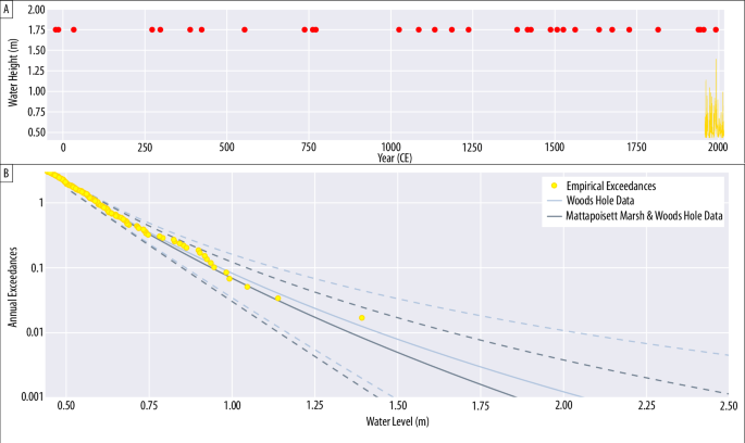
A Daily maximum tide gauge data from the Woods Hole tide gauge from 1957 to 2016 CE in yellow. Red dots show the mean values of ages for overwash deposits found in the published Mattapoisett Marsh record (Castagno et al.34). B In yellow, the empirical observations above the 99th percentile (0.43 m) of exceedance from the Woods Hole tide gauge. The light blue curves show the 50th percentile estimates with the 90% credible intervals for the expected number of exceedances per year calculated from model results using the Woods Hole tide gauge data only. The dark blue curves show the 50th percentile estimates with the 90% credible intervals for the expected number of exceedances per year calculated from model results using the Woods Hole tide gauge and the Mattapoisett Marsh (Castagno et al.34) geologic data.
In this case study, we use overlapping observations between the geologic and tide gauge records to provide two end member estimates for the geologic threshold and test two intermediate geologic thresholds. In doing so, we used a lower bound of 1.07 m, which is the water level recorded at the Woods Hole tide gauge from Hurricane Donna in 1960. This storm was not recorded by the geologic record at Mattapoisett Marsh34 and, therefore, presumably did not exceed the threshold required to create a geologic record. The upper bound was chosen to be 1.40 m, which is the most extreme water level recorded at the Woods Hole tide gauge from Hurricane Bob in 1991. A geologic record does exist for this storm in the Mattapoisett Marsh geologic record34, indicating Hurricane Bob did exceed the threshold required to create a geologic record. The geologic threshold estimated by the model was 1.29 m (90% credible interval: 1.15–1.38 m) (Supplemental Table 2). These estimates were within the bounds provided by water levels created by Hurricanes Donna and Bob at the Woods Hole tide gauge (1.07 and 1.40 m, respectively).
Compared to estimates based on the Woods Hole tide gauge alone, extreme water level estimates that incorporate geological data from Mattapoisett Marsh are modestly lower at the median but have greatly reduced uncertainty. This reduction in uncertainty arises through a reduction of the upper tail of estimates (Fig. 3, Table 2). For example, the 1% annual chance water level estimate shifts from a median (90% credible interval) of 1.44 m (1.17–2.04 m) to a 1.36 m (1.14–1.66 m) through the inclusion of the geological data: a 40% reduction in the width of the 90% credible interval. An even greater 48% uncertainty reduction happens for the 0.1% annual change water level estimate, which shifts from 2.06 m (1.49–3.65 m) to 1.86 m (1.44–2.56 m).
Cheesequake Marsh, New Jersey and The Battery, New York
We apply the model to a second case study using detrended daily tide gauge data from the Battery tide gauge over the years of 1920–2016 (https://tidesandcurrents.noaa.gov/datums.html?id=8518750) and a paleo-record of extreme water level events from Cheesequake State Park, New Jersey, USA35 (Fig. 4). The geologic record from Cheesequake State Park contains eight observations of extreme water levels in the form of overwash deposits35. The four youngest of the eight geologic observations are also observed in the Battery tide gauge record. Therefore, these four observations are treated as instrumental tide gauge data, while the four preceding observations are treated as geologic data in the model.
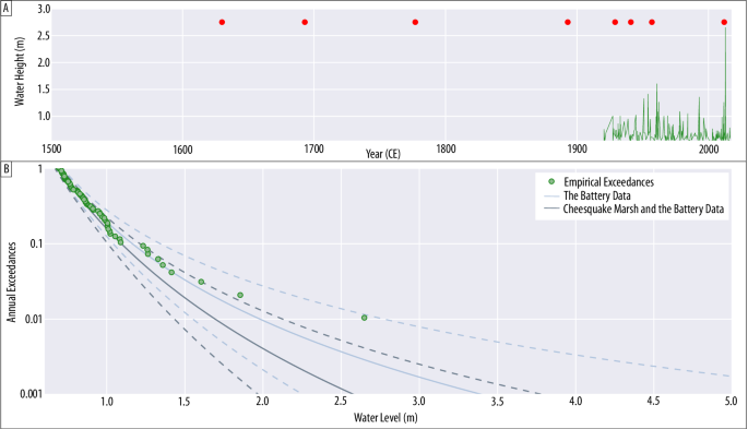
A Daily maximum tide gauge data from the Battery tide gauge from 1920 to 2016 CE in green. Red dots show the mean values of overwash deposits found in the Cheesequake record (Joyse et al.35). B In green, the empirical observations above the 99th percentile (0.54 m) of exceedance from the Battery tide gauge. The light blue curves show the 50th percentile estimates with the 90% credible intervals for the expected number of exceedances per year calculated from model results using the Battery tide gauge data only. The dark blue curves show the 50th percentile estimates with the 90% credible intervals for the expected number of exceedances per year calculated from model results using the Battery tide gauge and the Cheesequake (Joyse et al.35) geologic data.
Estimating the geologic threshold using overlapping observations in the geologic and instrumental records is not so straightforward in this case study. This is due to the fact that the Battery tide gauge record contains observations of extreme water levels that exceed in height some of those that are observed in the Cheesequake geologic record35. For example, an extratropical cyclone in mid-December 1992 created extreme floods from astronomical high tides combined with storm surges throughout the New Jersey and New York coasts. At the Battery tide gauge, this storm produced a maximum water level of 1.42 m above mean higher high water (MHHW). This storm did not produce an overwash deposit that is preserved in the Cheesequake geologic record, while other storms that produced lower water levels at the Battery tide gauge are recorded within the geologic record35. Without clear constraints for the geologic threshold from empirical data, we set wider bounds (0.8 to 1.6 m) for the model to estimate the parameter in this iteration. The geologic threshold estimated by the model was 1.51 m (90% credible interval: 1.37–1.59 m).
Even more so than in Massachusetts, the inclusion of geological data reduces extreme water level estimates through the thinning of the upper tail (Fig. 4, Table 3). The inclusion of geological data also results in a substantial lowering of median extreme water level estimates. For the 1% annual chance event, the water level estimate shifts from a median of 1.98 m (1.55–2.77 m) to 1.69 m (1.43–2.13 m). For the 0.1% annual chance event, the estimate shifts from 3.40 m (2.26–6.05 m) to 2.58 m (1.97–3.79 m): a reduction of over 0.8 m in the median and over 2.2 m at the 95th percentile. Notably, the inclusion of geological data shifts the estimates of Hurricane Sandy’s (2012) 2.7 m surge from occurring once every 376 years (92.3–3,130 years) to occurring once every 1,280 years (261–11,800 years).
The striking shift in return levels associated with events with an annual change of <10% is suggestive of non-stationarity between the period captured only by the geological record (1600–1920) and the period recorded by the tide gauge (1920 to 2016). Notably, the empirical exceedance estimates in the 1–10% range are more closely aligned with the curve estimated based on the tide-gauge data only than the fused curve (Fig. 4). Non-stationarity is also indicated by the geological record itself, which records as many events in the period from 1938 to 2018 as in the preceding three centuries. This non-stationarity could arise from a failure of the model assumption that the relationship between an event magnitude and preservation in the geological record is static in time; it could also reflect a climatological change leading to more extreme water level events in the 20th and 21st centuries than in the 17th–19th centuries.
Discussion
We develop a new statistical model with a POT framework that fuses tide gauge and geological data in order to test the utility of geologic observations in improving the precision of estimated extreme water level distributions. Previous studies have used extreme statistical theory to determine the return period of extreme water events from instrumental data alone8,11,36. Our model framework increases the number of extreme observations used in return period estimations over previous methods by including the noisy information stored in geologic records that are overlooked when instrumental records alone are used. The fusion of tide gauge and geologic data within this model framework greatly reduces the uncertainty of estimated extreme water level distributions, as demonstrated here using synthetic and published data, in particular by constraining the upper tail of estimates.
Other methods to increase the quantity of extreme water level data for return period estimation includes using synthetic storms from general circulation models and their respective modeled storm surges1,3,18. These storms and their respective surges are useful for understanding how changes to storm climatology can impact extreme water level return intervals3,18. However, these methods rely on global climate models and downscaling approaches to capture the relevant physical changes. On the other hand, data-driven methods have used historical data to reduce statistical uncertainties in estimating extreme coastal water level return period and to contextualize seemingly extreme outliers in instrumental data as predictable15,23. Investigations into the usefulness of historical data in frequency estimation originated in the field of hydrology24,25 to estimate the frequency of extreme fluvial flood events before being expanded into coastal environments.
This study is the first (to the authors’ knowledge) that extends data records beyond the historical period to incorporate proxy data from pre-historic storms to provide insight on extreme water level frequency. Other studies have also combined geologic evidence of storm-induced extreme water level events with evidence of paleo-climate forcing activity to provide insights on how storm climatology has affected storm surge levels in the past37,38,39. Insights from geologic data should further be used to validate and improve modeled storms tracks that are used to understand how the changing climate will impact storm surge recurrence intervals in the future.
The model currently assumes the probability of creating a geologic record of an extreme water level event relies solely on exceeding the geologic threshold. However, studies have shown that the relationship between the height of the geologic threshold and the likelihood of producing a geologic observation of extreme water level is more complicated40. For example, Joyse et al.35 found storms that generated extreme water levels captured in neighboring geologic reconstructions, such as a highly destructive and impactful unnamed 1821 Atlantic hurricane, were missing from the Cheesequake geologic record used as a case study in this work despite evidence of extreme flooding from the storm in the region. Reasons an extreme water level event could fail to be preserved in the geologic record include changes to coastal morphology over time, erosion of the overwash deposit by subsequent events, or bioturbation masking the overwash deposit’s signal29.
The model also currently assumes the relationship between the geologic threshold and the height of relative sea level (RSL) does not change through time, such that the probability of creating a geologic observation from the same extreme water level remains constant over time. This assumption is likely valid over the Late Holocene to the pre-industrial period, where coastal environments like salt marshes and mangroves have been able to accrete with relative sea-level rise41,42. While the temporally stationary version of the model works well for stable coastal environments over the last several thousands of years, it is not yet representative of coastal environments experiencing current and projected rates of RSL rise. In these instances, the difference between the height of the physical geologic threshold and the height of RSL would change through time.
Previous studies have incorporated changes to RSL in their estimations of extreme water level return periods calculated from tide gauge records by adding projections of RSL rise to historic return period curves19,43,44. Bulteau et al.23 account for changing RSL when incorporating historical data into their estimation of extreme coastal water levels in La Rochelle, France, by adjusting the perception thresholds in their model through time with the rate of RSL change. They assume RSL changes with global mean sea level throughout the historical period and use a local tide gauge to estimate RSL change over the instrumental time period of their data23. The thresholds for instrumental and geologic data in our model could similarly track RSL through time granted there is a geologic reconstruction of relative sea-level change in the region, as is the case with Cheesequake, New Jersey45. In order to incorporate the effects of changing RSL on extreme water level return periods, a temporally nonstationary version of our model needs to be adapted.
The case study using data from the Battery tide gauge and Cheesequake geologic record could be an example of where a nonstationary case of the model is needed. The mismatch between the tails of our modeled return period results and the most extreme water level events recorded at the Battery tide gauge (Fig. 4) suggests those most extreme water levels may occur less frequently than the tide gauge record reflects. It is unclear if the mismatch is a product of the tide gauge record being too short to capture the true frequency of these extreme events or due to the processes creating the extreme events at the tide gauge and in the geologic record being nonstationary in nature and, thus, not captured by our stationary model.
Relative sea-level rise along the mid-Atlantic coast, where the Battery tide gauge is located, has been rising faster than pre-industrial levels since the mid-19th century as a result of global ice melt and thermal expansion, glacio-isostatic effects, ocean-atmospheric interactions, and local land subsidence45,46,47,48. While we account for this increase in relative sea level by linearly detrending the Battery tide gauge data, changing storm climatology could be contributing to an increase in the height and frequency of extreme water level events through time3. Alternatively, non-stationarity in the geologic system could be driven by changes in the relationship between the height of relative sea level and the height of the dunes that act as the geologic threshold at the marsh (Fig. 5), which alter the preservational abilities of the marsh at Cheesequake through time. Whatever the cause, future iterations of the model need to incorporate the complicated relationship between the height of the geologic threshold and the probability of creating a geologic observation, including non-stationarity.
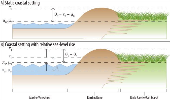
Notice from time ({t}_{0}) to ({t}_{1}) the relationship between RSL and the coast does not change. In this figure, the geologic threshold is represented by (tau) and the tide gauge threshold and equivalent location parameter for the model are represented by (pi) and (mu), respectively.
A nonstationary version of this model will have to account for how changes to RSL affect the probability of creating a geologic overwash event by exceeding the geologic threshold as the height of the threshold may not change at the same rate as RSL. Ideally, this version of the model would be adaptable to different coastal scenarios. For example, one scenario of interest may be a coastal environment that is not allowed to move in response to changes in RSL due to infrastructure or other mechanisms keeping the system in place. In this case, the height of the coastal barrier that must be exceeded to create a geologic observation would be held constant while RSL varies. Therefore, if RSL were rising, the difference between the height of the geologic threshold and the height of RSL would decrease, and it would become easier to produce a geologic observation through time. Nonstationarity could similarly be used to examine how return periods for extreme water levels change as the rate of RSL rise begins to outpace the rate at which salt marshes are able to accrete. In this scenario, the geologic threshold would move vertically at some fraction of the rate of RSL rise. Whichever combination of coastal environment and RSL scenario is desired, the temporally nonstationary version of the model needs to take into account variations in the height of the geologic threshold with respect to RSL.
We used a POT statistical approach to generate a Poisson Point Process model to estimate the expected number of annual exceedances for extreme water levels. We used synthetic data to demonstrate how the addition of geologic observations of extreme water levels, which provide no information regarding water height and have some degree of uncertainty in regards to time, improve return period estimates over using an instrumental tide gauge record, which are generally too short to observe many extreme water levels, alone. Our results show these geologic observations have the potential to greatly reduce uncertainties in extreme water level return period estimation by providing long-term data on the most extreme water level events that are often missing from instrumental records in desired numbers.
In addition to using synthetic data, we use two published geologic records of extreme water level events from Mattapoisett Marsh, Massachusetts28,34, and Cheesequake State Park, New Jersey35, fused with neighboring instrumental records from the Woods Hole and the Battery tide gauges, respectively, to test the applicability and effectiveness of our model. In using the real datasets, we show that geologic data improves estimates of extreme water level return periods, and we demonstrate how overlapping records between the two datasets can inform estimates for the geologic threshold. While Mattapoisett Marsh is one of the densest geologic records of extreme water level events, the sparser record from Cheesequake State Park shows smaller numbers of geologic observations can also reduce uncertainty in estimating extreme water level return periods.
Low-probability, high-impact extreme water level events from storms constitute the majority of risks and economic costs from natural hazards facing coastal communities. It is, therefore, consequential to marshal multiple lines of evidence to estimate the likelihoods of the occurrence of such events. Here, geologic data are shown to improve estimates for the return periods of extreme water levels when included with instrumental data. Incorporating nonstationarity and the probability of the geologic record preserving overwash events into the model will further allow risk assessments to adapt the model to mirror local coastal environments and to model under different RSL rise scenarios.
Methods
A Note on Stationarity
A central question in the interpretation of geological deposits in this framework is whether the magnitude of an event needed to produce an overwash deposit is stationary in time. Geologic records of extreme water-level events do not provide information regarding the position of the barrier and back-barrier systems with respect to paleo-relative sea level. Therefore, it is unknown if the likelihood of producing an overwash deposit from the same extreme water level changes with time. We model return periods under a temporally stationary model. In this model, the coastal environment, including the back-barrier and barrier systems, is assumed to accrete at the same rate relative sea level is rising (Fig. 5). There is evidence that, during the Middle to Late Holocene, sedimentation rates in salt marshes were able to keep pace with rates of relative sea-level rise41. With the relationship between the height of the coastal environment and relative sea-level held constant through time, the likelihood of creating an overwash events given an extreme water level of a specific height should remain relatively constant with time. In addition to failures of the assumption of a geological steady state, non-stationarity in the record could arise from a non-stationary climate (i.e., changes in the population characteristics of storms).
Statistical Model
We model occurrences of extreme water levels z (Table 4), which have exceeded some known threshold, with respect to time t, by a 2D Poisson point process with an intensity function ((lambda )) that takes the form of a density function of a Generalized Pareto Distribution (GPD)49:
where (mu), (phi), and (xi) are the model’s location, scale, and shape parameters, respectively7. The model parameters are estimated via Bayesian optimization using the Metropolis-Hastings Markov-Chain Monte Carlo (MCMC) in the ParaMonte Python library50. Bayesian inference allows for better accounting for and incorporation of uncertainty in model results. Classical likelihood methods (e.g., maximum likelihood estimation) do not fully account for model uncertainty, which can yield overly optimistic predictions of future extreme frequencies13,14,23,25.
For water levels (({z}_{0})) above a threshold such that their expected number of annual exceedances is substantially less than 1, the expected number of annual events ({N(z}_{0})) is given by:
Because tide gauge and geologic data are implicitly different in the extreme water-level information they provide, a unique likelihood function is applied for each data type. The likelihood functions are fused to estimate the model parameters when both tide gauge and geologic data are being used.
The likelihood function for the tide gauge data alone is the joint density function of all tide gauge observations at each water level ({z}_{i}) at time ({t}_{i}) above the tide gauge threshold for an extreme water level ((pi)) within the tide gauge’s observational time period of ({t}_{{present}}) (present day) to ({t}_{{tide}}) (beginning of the tide gauge record) and is given by:
where A is the number of tide gauge water level observations and (pi,>,mu)7,51. The first term is the product over all ({z}_{i}) for which ({t}_{{tide}} < {t}_{i} < {t}_{{present}}).
The likelihood function for geological data follows the form of the likelihood function for the tide gauge data while recognizing there is no water level data associated with the geologic data. Therefore, the likelihood function for the geologic data is the joint density function of the occurrence of geologic observations (({t}_{j}^{* })) above the geologic threshold (tau) within the geologic record’s observation time period of ({t}_{0}) (beginning of the geologic record) and ({t}_{{tide}}) (beginning of the tide gauge record) and is given by:
where B is the number of geologic water level observations. Note that (z) does not act as an observed water level in the integration above, which is consistent with the lack of water level associated with geologic records. When modeling with combined tide gauge and geological observations, the likelihood is given by the product of ({L}_{T}) and ({L}_{G}).
We assume the threshold to produce an extreme water level in the tide gauge record (pi) is known. We use the 99th percentile of the tide gauge data as the tide threshold, which for the synthetic data was 0.56 m and for the case studies was 0.43 and 0.54 m at the Woods Hole and Battery tide gauges, respectively19,43. Because the threshold that must be exceeded to produce a geologic observation, (tau), is unknown for real-world examples of geologic records, we allow the model to estimate the value of (tau).
Uniform prior distributions are placed on each of the model parameters. Values chosen to constrain the uniform distributions are chosen based on experts’ expectations for the true parameter values. For example, constraints of 0.40 to 1.00 were placed on the location parameter, (mu), given the expectation that (mu) should have a similar value to the tide threshold (pi), which for synthetic data was 0.56 m. Constraints on the uniform prior distributions for the scale and shape parameters were 100 to 500 and 10-10 to 1, respectively. The shape parameter for the GPD can be 0 or negative, but experience fitting this distribution to tide heights at other locations suggests negative values are unlikely for our region of interest along the eastern coast of the US19.
A uniform prior distribution is also used to estimate the value of the geologic threshold (tau) when geologic data are included in the optimization. For a synthetic data case, wide ranging constraints of 1.0 to 1.5 m are used (when the “true” value is known to be 1.35 m from the synthetic data generation process). For an empirical data case study, we review the overlapping time period between the tide gauge and geologic records to determine the bounds of the uniform prior distribution such that the largest extreme tide gauge observation that does not appear in the geologic record and the largest extreme tide gauge observation found concurrently within the geologic record serve as the lower and upper constraints on the uniform prior distribution, respectively.
A test was performed to determine how the tide gauge and geologic data each constrain the model parameters when the likelihood for the tide gauge and geologic data is used (e.g., the product of ({L}_{T}) and ({L}_{G})). To do this, we trained the model using three unique combinations of data. First, we trained the model using only tide gauge data; second, we trained the model using only geologic data; and third, we trained the model using a combination of tide gauge and geologic data. Results of these training tests can be found in the Supplemental Information (Supplemental Figs. 1–3).
Synthetic Data Experiments
To test the performance of the statistical model, we first apply it to synthetic data. The true extreme water-level distribution is assumed to follow a Student’s t-distribution, the parameters of which (mean = 0.8957, standard deviation = 199.2, degrees of freedom = 9.365) are chosen to fit de-trended daily maximum tide gauge data from the Battery tide gauge in New York City, USA (https://tidesandcurrents.noaa.gov/datums.html?id=8518750).
Within each set of synthetic observations, we first generate a 1000-year water-level record of daily maximum water-level observations sampled from the Student’s t-distribution (Fig. 2). We then create an observable 80-year tide gauge record from the final years of the 1000-year water-level record. The 80-year duration is consistent with the longest hourly tide gauge records on the eastern coast of the United States (https://tidesandcurrents.noaa.gov/datums.html?id=8518750) (Fig. 2). We use water levels above the 99th percentile of this 80-year tide gauge record as input to the model19,43. The observable tide gauge record has no uncertainties associated with water level or time.
Lastly, we create a geologic record of extreme water-level events associated with the highest water-level observations from the start of the 1000-year water level record (Fig. 2). To do this, we use a geological threshold of 1.35 m, representing the water level height an event must exceed to leave an overwash deposit. The threshold of 1.35 m was selected after several geologic thresholds were tested because it produced a realistic but higher number of geologic observations (11.3 ± 3.5 geologic observations over 1000 datasets). The geological record contains the timing of water events exceeding this threshold but does not record the water height. While the geologic threshold must be known to produce the synthetic geologic record, it is treated as an unknown parameter value when fitting the model.
To validate the model, we generated 1000 sets of synthetic data and used Bayesian optimization to estimate the parameter values for each dataset first using only the observational tide gauge data and second using the observational tide gauge and the geologic data13,23,25. We then calculated the 67 and 90% Bayesian credible intervals of the expected number of annual events at each water level given the optimized parameter values. Coverage ratios were estimated by finding the percentage of water levels within the 1000 synthetic datasets in which the true expected number of annual events for a given water level was within the 67 or 90% Bayesian credible intervals of the modeled annual event estimates47. In a robust model, the coverage ratio is expected to be 0.67 or 0.90 for the 67 and 90% Bayesian credible intervals, respectively52. Results estimated from the observational tide gauge record were compared with those estimated from the fused observational tide gauge and geologic records.
Case Studies
We selected two geologic records and their neighboring tide gauge records to apply our model to. First, we applied the model to data from a geologic record from Mattapoisett Marsh, Massachusetts28,34, and to water levels above the 99th percentile of tide gauge data from the neighboring Woods Hole tide gauge19,43. The Mattapoisett Marsh record was selected for its relatively high temporal resolution to give the model the most empirical data available for improving extreme water level return period estimates over using tide gauge data alone. We also selected data from a geologic record from Cheesequake, New Jersey35, and water levels above the 99th percentile of tide gauge data from the neighboring Battery, New York, tide gauge19,43. The Cheesequake record has a lower temporal resolution compared to the Mattapoisett Marsh record. The Cheesequake record is also located in a densely populated area that experienced extreme water levels during Hurricane Sandy in 2012. Therefore, the Cheesequake record provided an opportunity to test the model’s ability to improve extreme water level return periods with less data in an urbanized region with large investments in coastal development.
For the Massachusetts case study, we use Bayesian optimization to estimate the parameter values first using the Woods Hole tide gauge data alone and second using the Woods Hole tide gauge data in conjunction with the Mattapoisett Marsh geologic record. From the optimized parameter values, we calculated the 67% and 90% Bayesian credible intervals of the expected number of annual events for each water level of interest. Results of the return periods estimated from the Woods Hole tide gauge alone were compared to those estimated from the fused tide gauge and Mattapoisett Marsh geologic record. We follow the same methods in the New Jersey/New York case study when estimating model parameters and comparing the model using the Battery tide gauge data alone versus using the Battery tide gauge data fused with the Cheesequake geologic data as was used in the previous case study.


Responses