Multivariate compound events drive historical floods and associated losses along the U.S. East and Gulf coasts

Introduction
Compound flooding, resulting from multiple flood drivers such as precipitation, river discharge, and storm surge, poses a significant risk to coastal communities, now and in the future1. The interactions among flood drivers can lead to catastrophic socio-economic impacts that are often of longer duration and/or higher spatial extent2 than events caused by individual flood drivers3. These impacts are expected to be exacerbated by climate change (including sea-level rise along the coast) and urban development. Thus, assessments of socio-economic losses due to compound flooding events are a pressing concern4,5,6. These assessments require, however, comprehensive socio-economic loss records7, which are typically unreliable and/or largely unavailable8 along most coastal regions.
The United States (U.S.) is particularly vulnerable to compound flooding due to its exposure to different flood drivers combined with extensive coastal development and population density9. For instance, Hurricanes Harvey10,11 and Sandy12 evidenced how precipitation, storm surges, and ocean waves combined can have a drastic impact on coastal metropolitan areas. These events also exposed how vulnerable critical infrastructure is to compound flooding events9,13, emphasizing the urgent need for improved flood hazard assessment14 and risk mitigation and adaptation measures15,16. The U.S. East and Gulf coasts have been found to be major regional hotspots of historical and future compound flooding potential where associated impacts are projected to increase due to sea level rise and increasing storm activity1,9,13,17,18.
Despite the increasing risk of compound flooding, the underlying drivers of such events and their socio-economic impacts remain poorly understood7,16, particularly when compared to univariate flooding events. Identifying the nature of a particular flood event (i.e., compound or univariate) and its historical damage is challenging as it requires integrating different model datasets and socio-economic loss data, which usually come with large uncertainties9,19. To date, most assessments have focused on estimating the likelihood, intensity, and trends of compound flooding hazards (e.g., storm surges and precipitation) using statistical and process-based models9,19,20,21,22,23,24,25,26,27,28,29,30,31,32,33,34,35. It remains unknown how many of the historically observed flood events were compound events and which flooding drivers were involved in generating them. Furthermore, no link between such events and historically recorded direct damage has been established, particularly based on comprehensive, high-quality socio-economic loss data7,36,37.
We fill this gap by conducting an impact-based analysis using empirical loss data to quantify the socio-economic impacts of past compound flooding events along the U.S. East and Gulf coasts6,9,37,38,39. Here, we establish links between historical flooding events and their socio-economic losses for 203 coastal counties by combining meteorological, hydrological, and oceanographic data and flood loss information derived from the Spatial Hazard Events and Loss Database for the U.S. (SHELDUS40) between 1980 and 2018. We analyze the occurrence of compound flooding events, their underlying drivers and associated socio-economic impact for each coastal county. The results allow us to find regional hotspots of historical compound flooding, identify and contrast the drivers that caused them, and compare our results from this impact-based approach to those reported in previous studies that focused on compound flood potential using only flood driver information41.
Results
Spatial distribution of compound flooding events and their drivers
The U.S. experiences a considerable number of flooding events, with a total of 5506 recorded incidents in SHELDUS along the U.S. Gulf and East coasts between 1980 and 2018 (see Fig. S1). Figure S2 shows the total number of compound events, which are here defined as historical events. In this study, compound flood events are defined as those where at least two flood drivers exceed their 95th percentile thresholds simultaneously (see “Methods” section for more details). In Fig. 1, we show the ratio of compound events versus total number of flooding events (expressed in percent) and how this varies across counties. The results show that percentage values vary from 50% to 100% (Fig. 1). In 168 counties (across the 203 coastal counties analyzed), over 70% of the total recorded flood events were compound in nature. This means that in these counties, the majority of flood events involved at least two drivers. In all of the 203 counties, at least half of the recorded flood events were compound, indicating that compound flooding is a widespread phenomenon across the study region. The highest percentage of compound flooding events (ranging from 90% to 100%) occurred in counties along the U.S. Gulf Coast, from Louisiana to Florida’s Panhandle, and on the U.S. East Coast, between North Carolina and Delaware, and in Maine (Fig. 1). These are areas where most recorded flood events were caused by multiple flood drivers. For example, in Atlantic County (New Jersey) and in Gloucester County (Virginia) 90% and 100% of historical flood events were compound in nature, respectively. Furthermore, we find that compound event occurrence varies considerably between states, with Mississippi (MS) experiencing the highest percentage of compound flood events (89%), when averaged across all the counties, and Georgia (GA) having the lowest percentage (59.5%) (Fig. 1).

Gulf and East coasts. The inset panel shows the average percentage of compound flooding events for each state.
In Fig. 1, some counties, such as those in South Florida (e.g., Miami-Dade, Broward, and Palm Beach), show distinct color differences compared to their neighbors. These differences reflect localized variations in the proportion of compound flood events and the contributions of flood drivers. For example, Miami-Dade County recorded 30 flood events, of which 18 (60%) were compound. Precipitation contributed to 94.44% of these events, while river discharge (88.89%) and soil moisture (72.22%) also played significant roles, with relatively minor contributions from storm surge (5.56%) and wave height (5.56%). Similarly, Broward County experienced 24 compound events out of 26 total floods (92%), with precipitation as the dominant driver (100% contribution) alongside notable roles from river discharge (91.67%) and soil moisture (75%). Conversely, Palm Beach County reported 10 compound events out of 23 total floods (43%), with a more balanced contribution from drivers such as precipitation (70%), river discharge (80%), and storm surge and wave height (20% each). These localized differences are driven by unique geographic, hydrological, and oceanographic conditions that influence flood dynamics in these areas, as well as the location’s exposure and vulnerability profiles.
In Fig. 2, we show how often the different flood drivers were involved in creating the identified compound flooding events. The percentages shown (in Fig. 2) were determined by identifying instances where the respective flood driver exceeded its 95th percentile threshold during the identified compound flood events (see “Methods” for further details). We find that precipitation is most often a contributing driver, i.e., precipitation exceeded its 95th percentile threshold during 91% of all compound events (see “Methods”) (Fig. 2a). This highlights the importance of extreme rainfall events in creating compound flooding, including those caused by extra-tropical storms as well as hurricanes42,43. River discharge and soil moisture were also often involved in historical compound events for most counties (85% and 83% of all compound events, respectively) (Fig. 2b and c). The contribution of storm surge and ocean waves (described here as significant wave height) to compound flooding events varies considerably across space, with the highest percentage (ranging from 60% to 90%) in counties along the East coast between North Carolina and Maine (Fig. 2d, e).
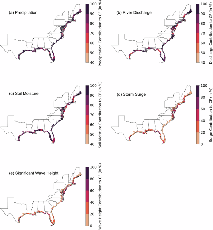
Spatial distribution of the frequency contribution (%) of different flooding drivers to compound events, a precipitation, b river discharge, c soil moisture, d storm surge, and e significant wave height. Drivers are considered to have contributed to a compound event when they exceeded their 95th percentile values (see “Methods” for more details).
Figure 3 shows more detailed results for the ten counties with the highest total number of recorded flooding events in SHELDUS. Doughnut charts show how often the different flood drivers contributed to compound events in these counties. For instance, in Harris County (Texas), precipitation exceeded its 95th percentile value during 119 out of the 155 total compound events. This highlights the county’s vulnerability to intense rainfall events, combined with other flood drivers, which, in this case, are often associated with tropical cyclonic storms and hurricanes. River discharge and soil moisture also played important roles, contributing to 114 and 102 compound events, respectively, indicating the substantial influence of upstream hydrological conditions and saturated ground on the generation of compound flood events and associated impacts. Soil moisture contribution is highest for Harris County, TX, and Charleston County, SC, and markedly lower for the other counties shown. Those same two counties also have the lowest fraction of compound events where oceanographic drivers (storm surge and wave height) contributed compared to the other eight counties.
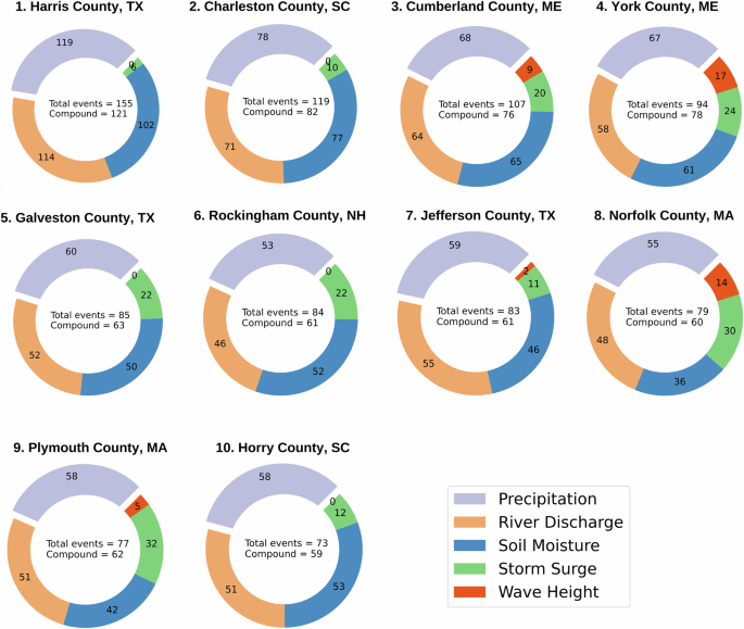
The county names are provided for each chart, and the total numbers of flooding events and compound flooding events observed within that county are presented. The colored segments represent the number of times each flood driver exceeded its threshold (95th percentile) during compound flooding events (see Methods for more details).
Clustering analysis of the impacts and drivers of compound flooding
To better understand regional patterns and similarities in the drivers of compound flooding, we performed a spatial cluster analysis. This approach allows us to identify groups of counties with similar flood driver profiles, providing insights into spatial variability and dominant mechanisms of compound flooding. Such an analysis is important for tailoring flood risk assessment and/or management strategies to the specific needs of different regions, especially given the diverse physical and climatic conditions along the U.S. East and Gulf coasts.
Through hierarchical clustering analysis of the relative frequency of contributions from different flood drivers (see Methods and Supplementary Fig. S3), we identify four key clusters where in each cluster, the counties exhibit, on average, similar percentages of occurrences in the different flood drivers during compound flooding events (see Fig. 4). As shown above, at the individual county level, precipitation, river discharge, and soil moisture (i.e., hydrological processes) have contributed to compound flooding more frequently than both storm surges and waves (i.e., oceanographic processes) in many counties; those counties are part of cluster 1 and stretch along the entire Gulf and East coasts (see Fig. 5). In clusters 2, 3 and 4, we find a higher occurrence of ocean waves and storm surge during historical compound flooding events compared to cluster 1, particularly in clusters 2 and 3 (>16%). These clusters are comprised of coastal counties mostly between North Carolina and New Hampshire, including Chesapeake Bay, and individual counties along the U.S. Gulf coast (Fig. 5), consistent with Fig. 2. We note that while clusters 2 and 3 look similar in Fig. 4 in terms of the average values of flood drivers across counties, the variability can still be very different and lead to the separation of clusters. For instance, counties in cluster 2 tend to have more uniform contributions from storm surge and wave height, while counties in cluster 3 show a wider range of values for these drivers. Because of this variation within clusters, they are treated as separate groups (Fig. S3). The dendrogram in Fig. S3 shows the hierarchical relationships between all counties and allows, for example, to further compare counties within our identified main clusters in terms of compound flooding drivers and how they relate to each other.
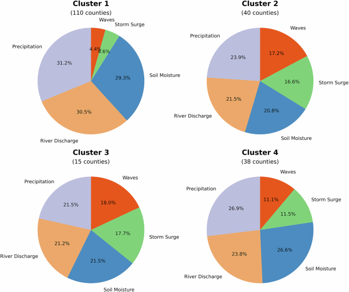
The frequency of each driver in each cluster has been normalized for a relative comparison.
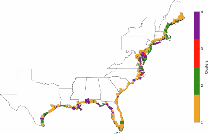
Each cluster is represented by a specific color as per legend.
Socio-economic impact of compound flooding and their regional distribution
Flooding events can lead to property (infrastructure) and crop damage. Figure 6 shows the percentage of historical property (Fig. 6a) and crop losses (Fig. 6c), recorded in SHELDUS, associated with compound flooding events as identified in our analysis. Over 80% of historical property and crop damage has been caused by events when multiple drivers were extreme (rather than univariate) in 92% and 81% of counties, respectively. For example, Orleans Parish, Louisiana, experienced property losses of ~US $24 billion between 1980 and 2018, almost entirely attributable to compound flooding (~99%), based on 29 compound events (out of 35 total recorded flooding events). Ocean County and Monmouth County in New Jersey have recorded over US$11 billion in flood damage with over 99% of this damage due to compound flooding. Those two examples from Louisiana and New Jersey also highlight the challenges when analyzing loss data that includes extreme outlier events. Hurricanes Katrina and Sandy were by far the costliest events in those counties, and both happened to be compound events where multiple flood drivers were extreme. Hence, it is not surprising that the majority of losses are linked to compound events. To account for this, we also derive the median losses from compound and non-compound events, and the ratio between the two, for all counties (Fig. 6b and d). A ratio larger than one indicates that compound events were more costly than non-compound events. For property losses, this is the case for 161 (out of 203) counties, and the average ratio across those counties is 26.68 (excluding the ones where no non-compound events were recorded, and a ratio cannot be calculated). This means that compound events (in terms of the median) were more than 26 times costlier than non-compound events; for crop losses that number increases to 76.02, further highlighting the damaging effects of compound flood events. Counties with ratios smaller than one indicate that non-compound events were more expensive. That is the case for 42 counties in terms of property loss and 28 counties for crop loss. Note that in some of those cases, the overall number of recorded flood loss events was small, and no compound events occurred, leading to a ratio of zero. Overall, these results show the widespread impact of compound flooding events on built infrastructure and agricultural assets along the U.S. Gulf and East coasts.
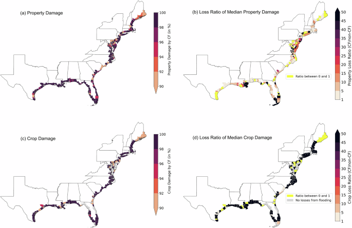
Percentage (%) of historical losses attributable to compound flooding for (a) property and (c) crop losses. The ratio between the median losses from compound and non-compound events for (a) property and (d) crop losses. The grey color indicates counties where there are no historical crop losses from flooding events. In (a) and (c) the colorbar is cut off at 90% and 25 counties with lower values are shown in the same color for property loss and 78 for crop loss. In (b) and (d), the colorbar is cut off at a ratio of 50 and 30 counties with higher ratios are shown in the same color for property loss and 115 for crop loss; this includes 16 counties for property loss and 110 counties for crop loss where no non-compound loss events exist and hence a ration cannot be calculated.
Discussion
Our study analyses the drivers of compound flooding events and their link to recorded socio-economic impacts (between 1980 and 2018) for 203 U.S. coastal counties. We find that ~80% of all flood events recorded along the U.S. Gulf and East coasts were compound (i.e., caused by multiple flood drivers) rather than univariate. In addition, despite finding considerable variability in the occurrence of these events across counties, at least 50% of total flood events in all counties were compound. These findings are consistent with previous work showing a relatively high likelihood of joint occurrence for different flood processes in these regions (e.g., rainfall and storm surge)9,22,23,24,28. Furthermore, historical compound flooding events in many counties were driven by more than two flood drivers, including multiple hydrological and oceanographic processes. This analysis underscores the critical roles of precipitation, river discharge, and soil moisture as dominant drivers of such events, while coastal processes such as storm surge and ocean waves contributed considerably to compound events certain regions and counties, but much less in others. The analysis, including empirical loss data, overcomes some of the limitations of previous work on compound event analysis where only certain pre-defined pairs of drivers were included and analyzed9,19,25,29,31,35,41,44,45,46,47,48,49,50.
Through clustering analysis, we identify different regions and counties with similar occurrences of different flood drivers during compound events. In further analysis, we find that most historical property and crop damage (more than 80% of total flood losses) have been due to compound flooding (rather than univariate) for more than 80% of the counties. This highlights the importance of considering and integrating compound flood event analysis, with all possible drivers, into hazard and risk assessments to support current and future adaptation and risk mitigation measures. This is particularly important since the coastal mean sea level continues to rise, and storm climatology with associated extreme weather events is projected to increase and intensify due to climate change along the U.S. Gulf and East coasts1,9,13. This could exacerbate future compound flooding events due to the intensification of one or more of their drivers.
The spatial distribution of coastal counties clusters along the U.S. East and Gulf Coasts shows important patterns, with several isolated counties exhibiting characteristics different from their surrounding regions. These clusters generally group counties with similar flood driver profiles, yet outliers can emerge due to different geographical features, historical storm impacts, or limited data samples. For instance, McIntosh County in Georgia emerges as an outlier of Cluster 3, despite being surrounded by Cluster 1 counties. This classification stems from only three recorded flood events, predominantly characterized by high contributions from waves and storm surges. Such cases underscore the importance of cautious interpretation when dealing with limited data points, as they may not fully represent the complete flood hazard profile of a county and can lead to apparent anomalies in spatial clustering analyses.
Despite the importance of our results, this study has some limitations. This includes, for instance, relying on multiple hindcast and reanalysis data sets (to overcome the lack of observational records in space and time), which may not adequately capture local extremes and their variability51,52,53. We also rely on historical flood event information from a county-level database (SHELDUS), which does not provide the exact location of the recorded impact. It is also important to highlight that the socio-economic impacts of such events are not only defined by the extreme flood drivers assessed here but are also dependent on vulnerability and exposure characteristics such as infrastructure resilience and population density54. Here, we define compound events based on the exceedance of the 95th percentile value by two or more drivers (see “Methods”), but other definitions are possible. To test the sensitivity of our results, we repeated the same analysis using the 99th percentile as a threshold (see Figs. S4 to S6). As expected, the number of compound events decreases but the overall conclusions drawn from the analysis are unchanged. Overall, our analysis indicates that research on the complex interactions between flood drivers and associated impacts needs to continue, including improved data for both the flood drivers and recorded losses as well as model development to explore unobserved events. The identification of different flood drivers during compound flooding events over different regions and counties, as shown here, suggests that a one-size-fits-all approach to compound flood risk assessment and forecasting may be inadequate.
Methods
Historical reanalysis/hindcast and socio-economic loss data
High-resolution data for five flood drivers (river discharge, precipitation, soil moisture, storm surge, and ocean waves) were obtained from multiple sources for 203 counties along the U.S. Gulf and East coasts. The data sets cover the period from 1980 to 2018 (Table 1). In this study, precipitation, storm surge, waves, soil moisture, and river discharge are considered as the primary drivers of compound flooding due to their distinct contributions to the initiation and evolution of such events. Following previous research55,56,57,58, soil moisture is considered here from one day before the flood event occurs, making it independent of the precipitation, river discharge and/or storm surge which ultimately resulted in the flood impacts. This approach ensures that soil moisture is not autocorrelated with these factors. For instance, high soil moisture can significantly reduce the infiltration capacity of the ground59, leading to rapid surface runoff during extreme precipitation events60. The other flood driver variables were considered in previous assessments of compound flood potential through dependence analysis19,28,35,41,46,61,62. Many of the variable combinations show some level of dependence because they can be caused by the same synoptic weather patterns or modulated in similar ways by teleconnection patterns. In some instances, one variable can be the response of the other, such as high discharge as a response of intense rainfall, but this would only happen near-simultaneously in certain small catchments with steep topography, while in many other instances, coincident rainfall in a downstream location and high discharge is the result of rainfall (often days earlier) further up in the drainage basin, snowmelt, or other factors including watershed releases. We also note that we rely here on reanalysis and hindcast data where models were developed to simulate the variables of interest, often without accounting for the influence of the other ones; for example, the hydrodynamic model used to derive storm surges does not account for river inflows along the coast, in the same way as the hydrologic model for discharge does not account for downstream storm surges. Hence, for the purpose of our analysis it is justified to assume that none of the flood drivers we consider are a direct response of the other, but they can still be correlated due to common links to weather phenomena and climate variability.
All data was re-gridded onto the precipitation spatial grid (~6 km) using the inverse distance weighted interpolation (Fig. 7). The data was temporally aligned to daily resolution. Historical direct property and crop losses ($USD) were extracted from the Spatial Hazard Events and Losses Database for the U.S. (SHELDUS) version 20 and cover 1980 to 2018. The SHELDUS data provides information on the hazard type (here, we only focus on flooding, which includes a total 5506 recorded flood events) and the start and end dates of the recorded impacts.
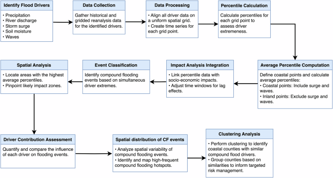
Methodology flowchart.
Classification of compound flooding and link to socio-economic losses
To provide meaningful comparison across space, we consider the relative extremeness of each flood driver based on the local climatology. To this end, we calculate percentile values at each grid point from the time series data (Table 1), thereby normalizing the data sets across space and time based on local climatology. This percentile-based approach enables us to evaluate the intensity of events in their local context, allowing meaningful comparisons across space and time while focusing on the most extreme occurrences. For each grid point in a county, we calculate the average of the percentile values for all flood drivers and select the grid point with the maximum value, which is assumed to correspond to the approximate location of the flood impact; SHELDUS only provides information at the county level with no exact location of the event available. For oceanographic drivers (storm surge and waves), percentile values are determined using the closest grid point to the coastline if our estimate of the impact location is within 6 km from the shoreline (i.e., coastal points) (note that 6 km is the resolution to which all other flood drivers were re-gridded). If a grid point is more than 6 km away from the shoreline, it is considered an inland point, where only precipitation, river discharge, and soil moisture are taken into account to estimate the impact location.
To classify historical flood events in SHELDUS as compound or non-compound, we identify instances where at least two flood drivers related to each flood event exceeded their 95th percentile values simultaneously, following previous work56. To link the flood drivers to socio-economic losses, we associate the flood drivers with the loss data in SHELDUS using a window of ±1 day. This allows us to account for short delays between the occurrence of extremes and their recorded impacts in SHELDUS. To avoid potential autocorrelation between soil moisture and precipitation and river discharge, we use soil moisture data from one day prior to each flood event when calculating percentile values. This ensures that soil moisture, which reflects cumulative hydrological conditions, is not directly influenced by precipitation or river discharge on the day of the flood loss event. By doing so, we reduce the overlap in timing between these drivers and provide a clearer assessment of their individual contributions to compound flooding. This approach allows us to link each extreme event identified in the historical model data to its recorded socio-economic loss data. The frequency of each flood driver during compound events was calculated by summing the number of instances when they exceeded their 95th percentile values. To assess whether our conclusions are robust against the choice of using the 95th percentile threshold, we conducted the same calculations considering the 99th percentile (see Supplementary Figs. S4–S6) as a threshold to define a compound event. This analysis only focuses on the most extreme occurrences of each flood driver. This sensitivity analysis is useful to validate our findings by ensuring that the identified patterns and relative contributions of the flood drivers remain consistent even when considering only the most severe events.
Identification of coastal counties with similar compound flood drivers
Hierarchical clustering was performed using Ward’s linkage method, a well-established approach that minimizes the total within-cluster variance62. This approach provides a robust framework for identifying and delineating counties with similar frequency of flood drivers into distinct clusters (Supplementary Fig. S3). We also determined the most frequent drivers in each cluster (Fig. 4). The data for the clustering included percentile values for the five flood drivers during compound events. This allows us to identify regional patterns and county-level similarities (Fig. 5). The initial cluster distances were computed using a multidimensional approach, where pairwise Euclidean distances (({D}_{{rm{i}},{rm{j}}})) were derived based on the percentile values of flood drivers for each county. This approach ensures that the clustering process identifies counties with high similarity in the frequency and magnitude of flood drivers during compound events.
where, ({D}_{i,j}) is the Euclidean distance between counties (i) and (j). This distance metric represents how similar or dissimilar two counties are in terms of the contributions from the flood drivers.
({x}_{i,k}) and ({x}_{j,k}) are the percentile values of the (k) th flood driver (precipitation, river discharge, soil moisture, storm surge, and wave) for counties (i) and (j), respectively, during compound events.
(k) is the index representing each of the flood drivers, where (k=1,,2,,3,,4,,5). corresponding to each flood driver, respectively.
(w) is the total number of flood drivers considered in the clustering.


Responses