Nitrogen dioxide (NO2) Meteorology and predictability for air quality management using TROPOMI

Surface nitrogen dioxide (NO₂) is a criteria air pollutant impacting the environment and public health. Major sources of nitrogen oxides (NOx ≡ NO + NO₂) include fossil fuel combustion, open biomass burning, and natural sources^1,2. In the atmosphere, volatile organic compounds (VOCs) are oxidized by hydroxyl radicals (OH), forming peroxy radicals (RO₂ or HO₂), which react with nitric oxide (NO) to produce nitrogen dioxide (NO₂). NO₂ can then be photolyzed to form ozone (O₃). Peroxyacetyl nitrate (PAN) forms when NO₂ reacts with acetyl peroxy radicals, while nitric acid (HNO₃) is formed when NO₂ reacts with OH. O₃ is a significant contributor to smog formation, while nitric acid contributes to acid rain^1,3.

Furthermore, NO₂ can transform into nitrates, contributing to particulate matter pollution, which is linked to respiratory diseases, premature deaths, and hospitalizations, especially in vulnerable populations^4,5,6. The World Health Organization (WHO) recently set a stricter annual exposure limit of 10 µg/m³ for NO₂ to mitigate these health risks⁷. Thus, accurate NO₂ monitoring and prediction are vital for effective air quality management.

However, traditional NO₂ monitoring methods are limited by high costs and complex operations, resulting in inadequate spatial data coverage^8,9. The short atmospheric lifetime of NO₂, coupled with its high spatial and temporal variability, complicates exposure assessments and highlights the need for regional scale monitoring strategies^10,11. Emerging tools like low-cost sensors (LCSs) offer affordable alternatives but often require frequent calibration due to accuracy issues^8,12,13,14. Satellite remote sensing provides extensive spatial coverage, with instruments like NASA’s Aura satellite and the Sentinel 5 Precursor used to study tropospheric NO₂ column trends over large areas^15,16. While these methods improve spatial resolution, combining satellite data with ground based measurements and predictive models can significantly improve forecasting surface NO₂ forecasting.

Considering the influence of weather conditions on NO₂ dispersion and transformations, leveraging meteorological data for NO₂ prediction could afford an innovative and cost effective approach^6,17. This study evaluates the potential of using local climatology to predict tropospheric NO₂ column concentrations, accounting for seasonal patterns and spatial distribution, providing a scalable solution for NO₂ monitoring in areas with limited measurement infrastructure.

Annual Mean Spatial NO₂ distribution

Significant variability in annual mean and year-to-year NO₂ distribution reaching (sim 4times {10}^{15}{rm{molecules}}{{rm{cm}}}^{-2}) from 2019 to 2023 is depicted in Fig. 1a–e, attributive to changes in anthropogenic activities, climate variability, and biomass burning events^18,19. Generally, NO₂ concentrations are highest over the most urbanized and industrialized capital i.e. Accra (5.559° N, 0.197° W). These areas are characterized by dense traffic, industrial activities, and higher population densities, contributing to elevated NO₂ emissions. Following 2019, particularly in 2020 (Fig. 1b) and 2021 (Fig. 1c), a relatively suppressed concentration is noticed, being partially explained by the impact of the COVID-19 pandemic, which led to reduced vehicular traffic, industrial slowdown, and a general decrease in fossil fuel combustion activities due to lockdown measures and reduced economic activities.

a–e Spatial distribution of the annual mean NO₂ column over Ghana for the years 2019–2023. Red areas indicate regions of higher NO₂ concentrations.

Full size image

The spatial distribution of NO₂ also shows regional variability, with higher concentrations generally detected in southern Ghana, where major cities like Accra and Kumasi are located. The coastal regions around Accra, consistently show higher NO₂ levels all-years-around likely due to the combined effects of traffic emissions, industrial activities, and maritime transport influences. The inland areas, particularly the northern regions, such as Tamale (9.403° N, 0.842° W) and Wa (10.060° N, 2.509° W), display comparatively lower NO₂ concentrations, reflecting the lower population density and less intensive industrial and vehicular emissions. The observed higher concentrations in urban areas are consistent with the known relationship between NO₂ and urban heat islands, where increased temperatures can enhance photochemical reactions, leading to higher levels of secondary pollutants like ozone (O₃) and PANs, as well as NO₂ itself^20,21.

Monthly and Seasonal NO₂ evolution

The seasonal NO₂ distribution depicted in Fig. 2a–d highlight distinct spatiotemporal variability for December to February (DJF), March to May (MAM), June to August (JJA), and September to November (SON) during 2019 to 2023. NO₂ column concentrations are at the peak during the DJF season across the study area, with pronounced levels around the highly urbanized and industrial regions like Accra. The elevated NO₂ concentrations during DJF is attributive to increased combustion activities, including open biomass burning, which is notably prevalent in the Savannah and arid areas during the dry season¹⁹. Furthermore, the DJF period in West Africa is characterized by stable atmospheric conditions, reduced convective activity, and minimal precipitation. These meteorological conditions limit the dispersion of pollutants, facilitating the accumulation of tropospheric column NO₂²².

The seasonal distribution of NO₂ across Ghana, highlighting variations during different seasons over the period from 2019 to 2023. a Mean NO₂ concentrations for December–February (DJF). b Mean NO₂ concentrations for March–May (MAM). c Mean NO₂ concentrations for June–August (JJA). d Mean NO₂ concentrations for September–November (SON). Red areas denote higher NO₂ concentrations, indicating potential hotspots for emission sources or stagnant atmospheric conditions.

Full size image

This seasonal pattern aligns with the MODIS burnt area map,¹⁹ which indicates that the DJF dry season corresponds to a period of heightened biomass burning and increased NO₂ emissions across the northern Savannah region, thereby contributing to elevated pollution levels. Moreover, the lack of convective mixing and a stable boundary layer during this dry season inhibit the vertical transport of pollutants, exacerbating the accumulation of NO₂. The transition to the rainy season during MAM (Fig. 2b) marks a significant shift in NO₂ distribution dynamics. Increased precipitation and convective activity characteristic of this period enhance pollutant dispersion, leading to reduced NO₂ column concentrations, particularly in the northern and central parts. Rainfall is an effective sink for NO₂ by facilitating wet deposition, while enhanced convection supports vertical mixing, thus diminishing NO₂ concentrations. However, despite the overall reduction, urban hotspots in the southern part, including Accra, continue to exhibit relatively elevated NO₂ levels, driven by persistent vehicular and industrial emissions.

The JJA season, being the peak rainy season, is marked by the lowest NO₂ concentrations (Fig. 2c). The frequent rain events, convective activities, and increased atmospheric instability characteristic of this period effectively remove NO₂ from the atmosphere through washout processes and enhance dispersion. Moreover, the wet and humid atmospheric conditions during JJA are less conducive to the formation and accumulation of NO₂, resulting in uniformly low values across all regions, including major urban areas.

During the SON season, the rains gradually subside (Fig. 2d), and there is a notable resurgence in NO₂ concentrations, particularly from the northern regions. The decline in rainfall frequency and the onset of more stable atmospheric conditions during this period reduce the efficiency of pollutant removal processes, facilitating a gradual accumulation of NO₂. Biomass burning activities, which tend to resume as conditions become drier, also play a significant role in the increasing NO₂ concentrations observed towards the end of the year. The seasonal transition observed during SON is likely influenced by regional meteorological dynamics, such as the Harmattan winds, which are prevalent during the dry down period and affect pollutant distribution and transport^19,21.

Figure 3 illustrates the fire activity observed by the MODIS Fire Radiative Power (FRP). The seasonal NO₂ distribution from December to February (Fig. 2a) aligns with increased fire activity observed in the MODIS FRP data (Fig. 3a). High NO₂ concentrations in the northern half during the dry season correspond with elevated FRP values, indicating significant NO₂ emissions from biomass burning. Conversely, lower NO₂ levels from March to August coincide with reduced fire activity, underscoring the key role of biomass burning in NO₂ variability, particularly during the dry season^19,22.

Fire activity patterns observed through MODIS Fire Radiative Power (FRP) for the seasons a DJF, b MAM, c JJA, and d SON during the period 2019–2022.

Full size image

Figure 4 presents the seasonality evaluation results, comparing NO₂ seasonality at selected stations using the Seasonality Index (SI) and monthly NO₂ column concentrations. Figure 4a shows Kete Krachi and Wa exhibit the highest SI values, signifying substantial seasonal variability in NO₂ levels. This variability connects strongly with seasonal biomass burning prominent during the dry season, as well as shifts in local meteorology. This trend is further corroborated by Fig. 4b, showing elevated NO₂ concentrations during the dry months (December to February). The high standard deviations for Kete Krachi (9.50 × 10¹⁴ mol/cm²) and Wa (7.76 × 10¹⁴ mol/cm²) further support this substantial variability, indicating significant month-to-month changes in NO₂ levels. In contrast, Axim has the lowest SI value among all the stations, indicating limited seasonal variation in NO₂ levels. Axim is a densely forested area situated in the rain hub of Ghana, and least urbanized and industrialized.

a Seasonality index comparison for selected stations and b time-series evaluation of monthly NO₂ column concentrations.

Full size image

Thus consistently low NO₂ levels reflects the absence of large scale anthropogenic activities, such as industry or dense vehicular emissions. This supported by Fig. 4b, where Axim shows minimal variation throughout the year, and by its low standard deviation (2.01 × 10¹⁴ mol/cm²). Whereas Kumasi and Accra show comparatively lower SI values than Kete Krachi and Wa (Fig. 4a), there is noticeable monthly variability (Fig. 4b). In particular, Accra exhibits pronounced increases in NO₂ concentrations during the dry months, suggesting that seasonal effects such as harmattan and biomass burning contribute to variations in NO₂. The standard deviations for Accra (5.89 × 10¹⁴ mol/cm²) and Kumasi (5.60 × 10¹⁴ mol/cm²) indicate considerable variability, reinforcing the observation that these urban centers experience dry seasonal peaks linked to both continuous and episodic emission sources.

The SI metric provides a useful indication of the degree of seasonality, while Fig. 4b shows that Accra, Kumasi, and Kete Krachi all exhibit peaks in NO₂ concentrations during the dry season. Thus, while the SI values for Accra and Kumasi are lower compared to Kete Krachi and Wa, indicating a blend of continuous emissions and seasonal influences, the monthly data in Fig. 4b highlight significant dry season peaks in these cities. This suggests that moderate SI values can represent meaningful seasonal changes, especially in urban regions where NO₂ sources are a mixture of continuous industrial emissions and episodic contributions like seasonal biomass burning. This highlights the significant impact of both meteorological conditions and seasonal biomass burning activities on NO₂ distribution in Ghana.

NO₂ and Meteorology relationship

To establish the meteorological conditions associated with the mean NO₂ concentration distribution as a proxy for NO₂ prediction, a correlation matrix for NO₂ at selected sites representative of the climatic zones with fourteen (14) climatological parameters is presented in Fig. 5.

Matrix displaying the correlation coefficients between NO₂ concentrations and local meteorological variables for selected locations in Ghana.

Full size image

In the Savannah zone, NO₂ concentrations show a negative correlation with average temperature, particularly in Wa (−0.33) and Tamale (−0.20). This suggests that elevated temperatures may enhance photochemical reactions, leading to increased NO₂ conversion into other species such as ozone. Moreover, higher temperatures can support stronger convective activity, resulting in more effective vertical redistribution of NO₂. The minimum temperature exhibits a strong negative correlation with NO₂ in both Wa and Tamale (−0.75 and −0.82, respectively), indicating that lower nocturnal temperatures might contribute to increased NO₂ levels, possibly due to temperature inversions that trap pollutants near the surface²³. The negative correlation with relative humidity in Wa and Tamale (−0.51 and −0.79) aligns with the expectation that higher moisture levels, often linked with precipitation and cloud cover, reduce NO₂ through wet deposition processes. Wind speed at both 2 meters and 10 meters shows a positive correlation in Wa (0.25 and 0.37) but a stronger positive correlation in Tamale (0.42 and 0.49), suggesting that higher wind speeds contribute to the dispersal of NO₂. The negative correlation with wind direction in both locations (−0.70 and −0.88) may reflect the influence of the prevailing monsoonal reversing wind patterns on pollutant distribution. Additionally, the negative correlation with cloud amount and precipitation in both stations suggests that these factors are crucial in reducing NO₂ levels in the Savannah zone.

In the Transition zone (Sunyani and Kete Krachi), NO₂ positively correlates with temperature (0.61 for average temperature and 0.69 for maximum temperature), suggesting that higher temperatures coincide with increased emissions, likely due to more intensive anthropogenic activities during warmer months. This increase in emissions appears to outweigh the photochemical loss of NO₂ that typically occurs at higher temperatures, leading to a net rise in observed NO₂ levels. However, the minimum temperature still shows a strong negative correlation (−0.80 in Sunyani and −0.88 in Kete Krachi), similar to the Savannah zone, indicating that cooler nights might lead to the accumulation of NO₂. The negative correlation with relative humidity is nearly perfect in Sunyani (−0.99), suggesting that high humidity significantly reduces NO₂ levels, likely through condensation and deposition processes. Wind speed shows a weak or negative correlation with NO₂, indicating that in the Transition zone, wind might not be as effective in dispersing NO₂ as it is in the Savannah zone. The strong negative correlation with wind direction, precipitation, and cloud amount reinforces the idea that these meteorological factors play a significant role in controlling NO₂ concentrations.

The Forest zone (Kumasi and Axim) exhibits a strong positive correlation between NO₂ and temperature, particularly in Kumasi (0.56 for average temperature and 0.65 for maximum temperature). This suggests that higher temperatures coupled with increased vehicular emissions and biomass burning, are linked to elevated NO₂ levels. However, the minimum temperature again shows a weaker negative correlation in Axim (−0.07), implying that nighttime cooling is less effective at trapping NO₂ in the Forest zone compared to other zones. The correlation with relative humidity is strongly negative in both Kumasi and Axim (−0.92 and −0.95), indicating that higher humidity, often associated with rain, reduces NO₂ concentrations significantly. Wind speed shows a consistent negative correlation with NO₂ in both stations, with Axim having a stronger correlation, suggesting that wind plays an important role in dispersing pollutants in the Forest zone. However, Axim shows a weak correlation with precipitation and solar radiation, reflective of local influencing factors such as proximity to the coast and vegetation cover.

Finally, the Coastal zone (Accra and Tema) reveals strong positive correlations between NO₂ and temperature, with both cities showing correlations above 0.60 for average temperature and maximum temperature. This may reflect the integrated effects of urban heat and local emissions, where higher temperatures coincide with increased NO₂ levels. The negative correlation with minimum temperature, though weaker than in other zones, suggests that nighttime cooling may help reduce NO₂ concentrations but is less effective in coastal cities. The correlation with relative humidity is strongly negative (−0.94 in Accra and −0.90 in Tema), indicating that higher moisture levels, which are common in coastal areas, play a critical role in NO₂ removal²³. Wind speed and direction also show strong negative correlations with NO₂, especially in Tema, highlighting the importance of coastal breezes in pollutant dispersion. The moderate positive correlation between NO₂ and solar radiation in Accra suggests that photolytic processes might also influence NO₂ levels in this region.

Meteorology based NO₂ Predictability

The predictive performance of the selected models for NO₂ columns across different climatic zones of Ghana (Savannah, Transition, Forest, and Coastal) is evaluated in Figs. 6, 7, and Table 1. The evaluation leverages statistical metrics including Mean Percentage Difference (MPD), Pearson’s correlation coefficient (r), and Willmott’s index of agreement (d) to assess how well the models can replicate observed NO₂ concentrations as captured by the TROPOMI instrument.

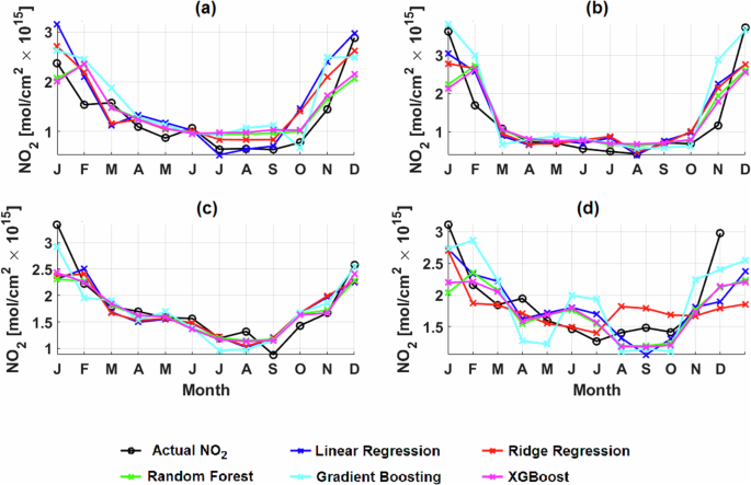
Predicted NO₂ concentrations across a Savannah, b Transition, c Forest, and d Coastal Savannah climatic zones using various meteorology-based models.

Full size image

Performance comparison of a Linear regression, b Ridge regression, c Random forest, d Gradient boosting, and e XGBoost models in predicting NO₂ concentrations across all four climatic zones.

Full size image

In the Savannah zone (Fig. 6a), all models exhibit reasonable accuracy, with MPD values ranging from 28.59 to 35.69%. Linear regression, Ridge regression, and XGBoost performed particularly well, each achieving MPD values under 30%, indicating smaller differences from the actual values. Pearson’s correlation coefficient (r) for these models remains high (0.84–0.89), with Willmott’s index (d) ranging between 0.87 and 0.92. This suggests that the models effectively captured the temporal variability of NO₂, though some bias remains in the seasonal prediction, particularly during the dry season, likely due to variable contributions from biomass burning. The Transition zone (Fig. 6b) presents a unique challenge. MPD values are notably higher than those in other zones, particularly for the Gradient Boosting model (37.76%), indicating challenges in accurately representing NO₂ concentrations. The correlation coefficients (r) are relatively consistent (0.81–0.89), but Willmott’s index (d) ranges between 0.85 and 0.93, showing that while temporal dynamics are somewhat captured, higher residuals may be indicative of complex interactions between emission sources and local meteorology that are less effectively modeled.

In the Forest zone (Fig. 6c), Random Forest, XGBoost, and Gradient Boosting models show improved performance compared to the simpler linear and ridge models. The Random Forest and XGBoost models have the lowest MPD values (10.11% and 9.87% respectively), demonstrating excellent predictive capability. High r values (0.92 and 0.91) and d values (0.92 and 0.91) also reflect their capacity to accurately capture temporal NO₂ patterns, particularly during transitions between the wet and dry seasons.

The Coastal zone (Fig. 6d) yields the lowest MPD values for Ridge Regression (13.84%) and XGBoost (15.35%), indicating that these models have relatively better predictive accuracy in this environment, likely due to more stable, continuous emission sources such as traffic and industry. However, the correlation coefficients (r) for all models in this zone are lower (0.66–0.75), and d values are also lower compared to the Forest zone, suggesting that capturing the variability in NO₂ emissions along the coast is inherently challenging. The influence of both anthropogenic and maritime factors leads to greater complexity, which may reduce model accuracy^24,25.

Figure 7 shows the scatterplots comparing predicted NO₂ concentrations to TROPOMI observations across all models and zones. Across all subplots (a–e), the highest consistency between predicted and actual values is observed for the Random Forest and XGBoost models, as indicated by the proximity of scatter points to the 1:1 line and higher r values. Conversely, Gradient Boosting shows larger discrepancies, which can be attributed to a higher sensitivity to hyperparameters and the risk of overfitting during model training.

Table 1 present summaries of the statistical results comparing the predicted and TROPOMI derived NO₂ based on the 20% monthly meteorology and NO₂ 2022 test dataset.

The evaluations presented, highlight that while the selected models especially with Random Forest and XGBoost provide improved predictability, there remain notable limitations related to model generalization across different climatic zones. The Forest zone benefits the most from these models, whereas the Transition and Coastal zones continue to pose significant challenges, primarily due to variability in seasonal meteorological conditions and diverse emission sources. In general, the assessment present the opportunity for further refinement in both model selection and hyperparameter tuning, especially for regions with complex emission and meteorological dynamics.

In summary, this study analyzed NO₂ distribution across Ghana (2019–2023) and evaluated statistical and machine learning models for predicting NO₂ concentrations, using TROPOMI NO₂ data and NASA POWER meteorology. Significant spatiotemporal variability was found, mainly due to anthropogenic activities, climate variability, and biomass burning. Elevated NO₂ levels were observed in urban areas like Accra, particularly during the dry season, influenced by emissions from traffic, industry, and biomass burning. Random Forest and XGBoost models showed strong predictive performance, especially in the Forest zone, while Transition and Coastal zones posed challenges due to complex meteorological and emission factors. Gradient Boosting was sensitive to hyperparameters and prone to overfitting, highlighting the need for careful tuning. Machine learning models offer potential for improved NO₂ predictions in regions with limited monitoring, but further model refinement and better representation of regional emissions and meteorology are needed to enhance prediction accuracy.

Study area geography and climatology

The study focuses on Ghana in Sub-Sahara West Africa, located at latitudes 4.5° N and 11.5° N and longitudes 3.5° W and 1.5° E, highlighted by the dashed outline in Fig. 8. This geographic location positions it within the tropical climate zone, characterized by distinct wet and dry seasons. The climate varies significantly across the country, influenced by the interplay between the dry, dust laden Harmattan winds from the Sahara Desert to the north and the moist maritime air from the Gulf of Guinea to the south^26,27.

Map showing Ghana’s position in West Africa, highlighting the four main climatic zones (Savannah, Transition, Forest, and Coastal Savannah) and selected synoptic stations.

Full size image

Ghana’s climate can be categorized into four main zones: the Savannah, the Transition, the Forest, and Coastal Savannah (Fig. 8). The Savannah zone, located in the northern part of the country, experiences an unimodal rainfall pattern from May to October. The Transition zone, located centrally, marks a shift between the unimodal rainfall in the north and the bimodal rainfall pattern found in the southern Forest zone. The Forest and Coastal Savannah zones, covering the southern part of Ghana, experience two distinct rainy seasons, from March to July and September to November, interspersed with short dry spells. These variations in rainfall patterns, temperature, and humidity across the country present diverse environmental conditions for atmospheric NO₂ dispersion and transformation^28,29. Selected cities representative of the climate zones and synoptic stations under the Ghana Meteorological Agency, relevant for discussions are highlighted as black dots in Fig. 8.

The climatology is further characterized by its temperature regime, with average temperatures ranging between 21 °C and 32 °C. The coastal areas typically exhibit higher humidity levels and more stable temperatures due to the moderating influence of the Atlantic Ocean. In contrast, the northern Savannah region experiences more extreme temperatures and lower humidity levels, contributing to different atmospheric chemical processes and pollutant dispersion dynamics^23,30,31. For example,Ogen²³ showed that positive vertical airflow indicative of downward air movement suppressed the dispersion of NO₂ over Western Europe.

Understanding NO₂ distribution requires considering both regional meteorological conditions and localized factors influencing air quality. This study leverages this geographic and climatic diversity to assess NO₂ dynamics, using a combination of satellite data and meteorological parameters to enhance predictive modeling capabilities for air quality management in Ghana.

TROPOMI Nitrogen Dioxide (NO₂) data

The TROPOspheric Monitoring Instrument (TROPOMI), launched on 13 October 2017 as part of the European Space Agency’s Sentinel 5 Precursor satellite mission, provides high resolution measurements of atmospheric NO₂ column. Operating in a sun synchronous, low earth orbit (825 km altitude) with a 13:30 local solar time equator crossing, TROPOMI achieves daily global coverage with a 2600 km swath width and a pixel resolution reduced to 3.5 × 5.6 km² at nadir after August 2019^21,32. This passive optical sensor relies on solar UV visible radiation, capturing radiance in the 405–465 nm spectral window to derive NO₂ column amounts through differential optical absorption spectroscopy³³.

The NO₂ retrieval process involves converting top-of-atmosphere spectral radiances to slant column densities, followed by separating the tropospheric and stratospheric components using the TM5-MP model and applying air mass factors (AMF) to estimate the vertical column content. The AMF calculation, which influences the retrieval’s accuracy, is sensitive to factors such as surface reflectance, NO₂ vertical profiles, and atmospheric scattering. While there is some significant bias (ranging from 20 to 40%) in urban areas due to uncertainties in air mass factor (AMF) calculations, as well as additional uncertainties from other factors such as fitting errors, stratospheric assumptions, and surface reflectance, TROPOMI’s data remains valuable for analyzing trends in NO₂ column^34,35,36,37.

For this study, we utilized monthly averaged NO₂ data from the NASA Health And Air Quality Applied Science Team (HAQAST) Level 3 GLOBAL TROPOMI NO₂ collections (Version 2.4) at a 0.1° × 0.1° resolution from 2019 to 2023, which provides good spatial and temporal coverage suitable for integrating with NASA’s climatology products to evaluate NO₂ meteorology, for modeling and prediction of NO₂ levels in Ghana. The data is accessible at: https://search.earthdata.nasa.gov/search?q=HAQ_TROPOMI_NO2_GLOBAL_M_L3.

The MODIS burnt area data presented by Kugbe¹⁹ indicates that biomass burning significantly contributes to NO₂ levels over Ghana. To further highlight the impact of biomass burning on NO₂ distribution, we retrieved Fire Radiative Power (FRP) data from NASA’s Fire Information for Resource Management System (FIRMS). The FRP data, derived from MODIS Aqua/Terra, was used for comparison with NO₂ data, covering the period from 2019 to 2022.

Meteorological Data from NASA POWER

A collage of recent 30 years of climatological reanalysis products comprising 14 parameters was retrieved from the National Aeronautics and Space Administration Prediction of Worldwide Energy Resource (NASA POWER) agro-climatological online data viewer service system at 0.5° grid area (https://power.larc.nasa.gov/data-access-viewer/). The products consisted of Temperature at 2 m (^oC), Relative Humidity at 2 m (%), Wind Direction at 2 m (Degrees), Wind Speed at 2 m (m/s), Wind Speed at 10 m (m/s), Maximum Temperature at 2 m (°C), Minimum Temperature at 2 m (°C), Maximum Wind Speed at 2 m (m/s), Minimum Wind Speed at 2 m (m/s), Cloud Amount (%), Maximum Wind Speed at 10 m (m/s), Minimum Wind Speed at 10 m (m/s), Total Rainfall (mm), and All Sky Surface Shortwave Downward Irradiance (MJ/m²/day).

A detailed description of NASA POWER and extensive validation of the cloud and radiation products over Ghana were presented by Asilevi Junior²⁵ and Quansah,³⁸ showing Willmott’s index of agreement between 0.7 and 0.99 ± 0.01. Alongside, several works have represented NASA POWER’s suitability and adaptability for the region of interest^26,39,40,41.

In this work, the spatial coverage of NASA POWER data was adapted as the regional climatological framework to evaluate the NO₂ meteorology and subsequently develop the meteorology based NO₂ prediction.

Seasonality Index (SI) and NO₂ Predictive Models

Based on the periodicity of NO₂ data, the Seasonality Index (SI) by Walsh and Lawler⁴² was adapted as a test tool to ascertain the strength of NO₂ seasonality. This is to ensure that NO₂ has a predictable pattern. The SI is a computational tool developed to quantify the intra-annual distribution of climatic data, which several authors have used for rainfall seasonality studies^43,44,45. In the context of NO₂, the SI can be adapted to measure the degree to which NO₂ columns fluctuate throughout the year. A higher SI indicates that NO₂ columns are concentrated in a few months of the year (high seasonality), while a lower SI suggests that NO₂ levels are more evenly distributed across the year (low seasonality). The SI is computed by Eq. 1, where ({{rm{R}}}_{{rm{i}}}) is the total NO₂ concentration for year i, ({{rm{x}}}_{{rm{in}}}) is the NO₂ concentration in month n for year i.

The prediction of NO₂ column concentrations leverages a combination of statistical and machine learning models to integrate satellite derived NO₂ column data from TROPOMI with climatological data from NASA POWER. The primary goal is to establish a predictive framework that captures the dynamic interactions between local meteorological conditions and NO₂ levels, providing a scalable solution applicable for monitoring air quality in regions with limited ground based measurements. To achieve this, the study utilizes multiple modeling approaches, each tailored to capture different aspects of the relationship between NO₂ column concentrations and meteorology.

Linear regression is first employed to establish a foundational model that describes the linear relationship between NO₂ columns and meteorological predictors, such as temperature, relative humidity, wind speed, precipitation, solar radiation, and cloud cover. The linear regression model is represented mathematically by Eq. 2:

where β₀ is the intercept, β₁, β₂, …, β_n are the coefficients for the predictors X₁, X₂, …, X_n, and ε is the error term. While linear regression provides a baseline understanding, it may not fully capture the complex, nonlinear interactions between meteorological variables and NO₂ levels⁴⁶.

To address potential nonlinearities and multicollinearity among predictors, ridge regression is applied as an extension of linear regression. Ridge regression introduces a regularization parameter that penalizes the size of coefficients, thus reducing model complexity and mitigating overfitting^47,48. The ridge regression objective function is:

where λ is a regularization parameter controlling the degree of shrinkage applied to the coefficients. This regularization helps stabilize the estimates when predictors are highly correlated, ensuring more reliable predictions.

For capturing complex, nonlinear interactions between the predictors, random forests are employed. Random forests are an ensemble learning method that constructs multiple decision trees during training and outputs the mean prediction of the individual trees. Each tree in the ensemble is built from a random subset of the data, allowing for diverse decision boundaries and improving the model’s generalization capabilities⁴⁹.

Gradient boosting is another ensemble learning method applied in this study to further refine NO₂ predictions. Unlike random forests, gradient boosting sequentially builds a series of decision trees, where each new tree corrects the errors made by the previous ones. The method minimizes a specified loss function by adding new models that predict the residuals of prior models, leading to highly accurate predictions⁵⁰. The model is represented by Eq. 4:

where F_m(x) is the current model, F_m-1(x) is the model from the previous step, h_m(x) represents the new decision tree added at stage m, and γ_m is the learning rate. This iterative approach allows the model to focus progressively on the hardest-to-predict data points, enhancing overall performance.

XGBoost, an optimized version of gradient boosting, is also utilized for its overall computational efficiency and improved accuracy. XGBoost incorporates both first and second order derivatives in its optimization process, which allows for faster convergence and better handling of complex data patterns^51,52. The function representation at step t is:

where ({{rm{f}}}_{{rm{k}}}left({{rm{x}}}_{{rm{i}}}right)) and ({{rm{f}}}_{{rm{t}}}left({{rm{x}}}_{{rm{i}}}right)) are the prediction values for the k and t iterations of the XGBoost model respectively; ({{rm{f}}}_{{rm{i}}}^{({rm{t}})}) and ({{rm{f}}}_{{rm{i}}}^{{rm{t}}-1}) are the prediction values for the tth and t-1th iterations of the ith sample; ({{rm{x}}}_{{rm{i}}}) is the input variable. Additionally, XGBoost includes regularization techniques to further prevent overfitting, making it particularly suitable for predicting NO₂ concentrations for diverse geographical regions.

The models were trained on a dataset comprising monthly meteorological variables and corresponding NO₂ column concentrations, capturing the local climatology’s influence on pollutant dispersion and transformation processes. Specifically, the data was split such that 80% was used for training and 20% was used solely for validation, ensuring that at least 20% of the data was not seen by the model during training. This approach allows for an accurate evaluation of the model’s ability to predict NO₂ concentrations when exposed to unseen data, reflecting real world performance. The training dataset comprised the years 2019–2021, while the validation dataset comprised the year 2022. The integration of meteorological observations represents a novel approach to NO₂ monitoring, offering a scalable solution for air quality management.

Statistical and correlation tools

To assess the correlation between NO₂ column and meteorology, as well as the performance of the prediction models, Root mean square difference (RMSD), Mean bias difference (MBD), and Pearson’s correlation coefficient (r) for n observations presented in Eqs. 6 to 8 are used where RD is the residual difference between predicted ({{rm{NO}}}_{2,{rm{predicted}}}) and observed ({{rm{NO}}}_{2,{rm{Observed}}}), and σ is the standard deviation^53,54.

The RMSD is a standard statistical measure of the variation margin between observed and predicted data, for which zero in the ideal case and a smaller metric indicative of a low marginal difference⁵⁴. The MBD offers a statistical measure of the spread of estimation from observation, with near zero MBD values being desirable. The Pearson’s correlation coefficient (r) was used to measure the strength of NO₂ and local climatology correlation²⁵.