Noise-agnostic quantum error mitigation with data augmented neural models

Quantum technologies have potentially disruptive applications in the fields of computing, communication, and sensing. In the near term, however, the demonstration of practical quantum advantages remains challenging due to the presence of noise. A promising technique to restore quantum advantages in realistic noisy devices is quantum error mitigation¹, including zero-noise extrapolation (ZNE)^2,3,4,5,6, Clifford data regression (CDR)^7,8,9,10, probablistic error cancellation^2,11,12, and virtual purification^13,14,15.

A limitation of the existing error mitigation methods is that they generally require prior knowledge about the noise model, leading to an overhead in terms of noise characterization operations^16,17,18. A promising approach to circumvent this issue is to exploit deep neural networks, which have been successfully applied to other quantum tasks such as quantum state characterization^{19,20,21,22,23}, quantum property estimation^24,25, quantum verification^26,27, and quantum simulations^28,29. Previous research^30,31,32 has also explored the use of machine learning models to estimate the output fidelity of quantum circuits. Although these approaches do not eliminate noise in the circuit output, they hold promise in guiding the generation of quantum circuits with fewer errors. Recently, a series of works explored the application of deep neural networks directly to quantum error mitigation^33,34,35,36. Nevertheless, training these networks generally requires access to noise-free data, which can be hard to obtain from experiments or from classical simulations.

Here we propose a neural model that achieves quantum error mitigation without prior knowledge of the noise and without any access to noise-free data. To achieve this feature, we introduce a technique, called quantum data augmentation, to expand the original data set by generating new data from a fiducial set of noisy processes. Our technique provides a quantum version of classical data augmentation techniques^37,38, which have proven valuable in scenarios where the available training data is limited^39,40.

Our model exhibits four major features. (1) No need of noise-free statistics from the target quantum process. Thanks to this feature, our model is applicable to relevant real-world scenarios where the ideal target process is hard to simulate. (2) Noise-agnostic error mitigation. The model does not require prior knowledge about the noise model, nor about the values of the noise parameter. As a result, it avoids overheads due to noise characterization, and works both for Markovian and non-Markovian types of noise. (3) Versatility. The model works in a broad range of applications and enables error mitigation for quantum algorithms, dynamics of many-body systems, and continuous-variable quantum information processing. In addition, it accepts the input data in a variety of different forms, including expectation values of quantum observables, statistics of measurement outcomes, and estimates of the Wigner function. (4) Transferability. The trained model exhibits the capability to mitigate errors for circuits sharing the same circuit skeleton as those considered in the training, all without the need for retraining. This feature makes it possible to apply the model to a wide range of quantum circuits, enhancing its practical utility and scalability. To demonstrate these features, we test our model on a series of paradigmatic quantum algorithms, such as variational quantum eigensolvers⁴¹ and quantum approximate optimization⁴², and quantum dynamics, such as the many-body dynamics of the Ising model and the Kerr Hamiltonian⁴³ for continuous variable systems. Furthermore, we tested our model on real quantum hardware. The results demonstrate its superior performance compared to previous methods, including ZNE and CDR.

The DAEM model

Let us start by specifying our error mitigation framework. We consider a target quantum process ({mathcal{E}}) corresponding to a quantum circuit composed of a specific sequence of single-qubit and CNOT gates (which is general as single-qubit gates and CNOT gates can form a universal gate set), with the restriction that only Pauli measurements are performed. The circuit represents the action of an ideal quantum device in the absence of noise. Note that our method also applies to some reversible processes without explicit circuit representations (see “Error mitigation for continuous-variable processes”). In the real world, however, one has only access to noisy versions of the process ({mathcal{E}}). Such noisy versions will be denoted by ({{mathcal{N}}}_{lambda }({mathcal{E}})), where ({{mathcal{N}}}_{lambda }) represents the noise model and λ indicates the noise parameter. The input state of the process ({{mathcal{N}}}_{lambda }({mathcal{E}})) is randomly selected from an ensemble ({mathcal{S}}={{{rho }_{s}}}_{s = 1}^{n}), which can generally contain multiple quantum states. For every input state ({rho }_{s}in {mathcal{S}}), the goal of error mitigation is to estimate the statistics of measurements performed on the ideal output state ({mathcal{E}}({rho }_{s})) given access to data from its noisy version ({{mathcal{N}}}_{lambda }({mathcal{E}})({rho }_{s})).

Here we focus on a set of Pauli measurements ({mathcal{M}}) of interest, such as a set of Pauli measurements performed on a subset of the output qubits in a quantum computation. Each measurement ({{boldsymbol{M}}}_{i}={({M}_{ij})}_{j}) in ({mathcal{M}}) is a positive operator-valued measure consisting of m positive operators that satisfy the normalization condition (mathop{sum }nolimits_{j = 1}^{m}{M}_{ij}={mathbb{1}}). This general setup covers tomography (when ({mathcal{M}}) is informationally complete), as well as quantum algorithms, where a single measurement is used for read-out.

To achieve error mitigation, we now introduce a neural network-based model. Our model, called data augmentation-empowered error mitigation model (DAEM), is illustrated in Fig. 1. Its high-level structure consists of two phases. In the first phase, the Noise-Awareness phase, we train a neural network to remove the action of the noise ({{mathcal{N}}}_{lambda }) from the measurement statistics. The training is boosted by a technique called quantum data augmentation. The key idea is to train the network on data generated by fiducial processes, a set of quantum circuits derived from the target quantum process.

The entire procedure is divided into two phases. In the first phase, known as Noise-Awareness phase, we train the neural model for error mitigation with the assistance of a fiducial process responsible for data augmentation. In the second phase, known as Error-Mitigation phase, we apply the trained neural model to mitigate the errors in noisy measurement statistics collected from the noisy version of the target quantum process.

Full size image

The fiducial process ({mathcal{F}}) is expected to have two desired features: First, in the absence of noise, a classical computer should be capable of efficiently generating adequate measurement data corresponding to various input states and Pauli measurements. In the presence of noise, the fiducial process ({{mathcal{N}}}_{lambda }({mathcal{F}})) should be implementable using the same quantum computing hardware that executes the target process. Second, when implemented on the quantum hardware, the noise pattern of the fiducial process should be as close to that of the target process as possible. This ensures that error mitigation techniques learned on the fiducial process can be effectively transferred to the target process.

Following this spirit, we construct the fiducial process by making changes to the execution of the original implementation according to the following recipe: (1) For every single-qubit gate R, we instead ask the quantum computer to execute (sqrt{{R}^{dagger }}sqrt{R}), which equals an identity gate in the ideal case. The motivation for this is to make the noise pattern of the fiducial process emulates that of the target process. For example, in trapped ion systems, the replaced gates can be implemented with the same execution time by adjusting the duration of the interaction. This leads to similar noise patterns assuming the dissipative part of the qubit dynamics to be fixed. Note that the implemented fiducial process will not be an identity process in general, since the implementation is not perfect. (2) All CNOT gates are executed according to the original circuit.

With this recipe, since ({mathcal{F}}) consists only of CNOT gates, the measurement statistics for the output state ({mathcal{F}}(sigma )) with respect to Pauli measurements can be efficiently computed for any product state σ: Note that ({mathcal{F}}) is Clifford since it consists of CNOTs only. Taking the Heisenberg picture, the evolution of any Pauli observable P under ({{mathcal{F}}}^{dagger }), which results in an N-qubit Pauli observable ({{mathcal{F}}}^{dagger }(P)), can be efficiently simulated. Since σ is a product state, the desired expectation ({rm{tr}}({{mathcal{F}}}^{dagger }(P)sigma )) can be computed classically in O(N) time.

To generate the training data, the experimenter collects measurement statistics by executing the noisy fiducial processes ({{mathcal{N}}}_{lambda }({mathcal{F}})) on a set of product states {σ_s}, using the same hardware as the target quantum process. The acquired measurement statistics will be denoted by ({{{{boldsymbol{p}}}^{{prime} }}_{i,s}^{(1)}}), while the ideal measurement statistics will be denoted by ({{{boldsymbol{p}}}^{{prime} }}_{i,s}^{(0)}:= {({rm{tr}}({mathcal{F}}({sigma }_{s}){M}_{ij}))}_{j}). In scenarios where varying the noise is possible, statistics can also be collected with various noise parameters ({{{lambda }_{k}}}_{k = 1}^{K}). In such cases, the acquired measurement statistics are denoted by ({{{{{boldsymbol{p}}}^{{prime} }}_{i,s}^{(k)}}}_{k = 1}^{K}). Note that we do not assume knowledge of the exact values of ({{{lambda }_{k}}}_{k = 1}^{K}) and, consequently, do not require any extra noise estimation procedure. We then train the neural model by providing tuples of the form ({({{{boldsymbol{p}}}^{{prime} }}_{i,s}^{(k)})}_{k = 1}^{K}) corresponding to a given input state σ_s and a given measurement M_i. Thanks to the aforementioned features of the fiducial processes, the ideal statistics ({{{boldsymbol{p}}}^{{prime} }}_{i,s}^{(0)}) can be computed efficiently from the input product state σ_s. In the training, we optimize the parameters of the model with respect to a loss function ({mathcal{L}}) that quantifies the deviation between the predicted statistics and the noise-free one (see “Methods” for details).

After the training is concluded, the model can be used for error mitigation on the target process ({mathcal{E}}). The experimenter collects measurement statistics by performing the noisy process ({{mathcal{N}}}_{lambda }({mathcal{E}})) on an arbitrary input state (rho in {mathcal{S}}), with different noise parameters ({{{lambda }_{k}}}_{k = 1}^{K}). The corresponding statistics will be denoted by ({{boldsymbol{p}}}_{i}^{(k)}={({rm{tr}}({{mathcal{N}}}_{{lambda }_{k}}({mathcal{E}})(rho ){M}_{ij}))}_{j}). The neural model then outputs the inferred ideal statistics ({{boldsymbol{p}}}_{i}^{(0)}:= {({rm{tr}}({mathcal{E}}(rho ){M}_{ij}))}_{j}) pertaining the target process ({mathcal{E}}). A detailed description of the implementation of the neural model in various examples is provided in the “Methods” section.

An important feature of the DAEM model is that it can be applied to ensembles containing multiple input states. In addition, the states appearing in the Error Mitigation phase do not need to be the same states used in the training. Furthermore, it is worth stressing that the model does not require any ideal measurement data (neither experimentally generated nor classically simulated) for the target process ({mathcal{E}}). As a consequence, it has the potential to be applied to large-scale systems where the classical simulations are not feasible, and realistic experiments are affected by non-negligible amounts of noise.

Additionally, our model can be trained for multiple target processes that share the same circuit skeleton but have different parameters. This is achieved using a set of fiducial processes. The underlying intuition is that circuits with the same skeleton are likely affected by similar noise patterns. Consequently, the knowledge gained from mitigating errors in one such circuit can be transferred to others within the same structural framework. This transferability enhances the efficiency and applicability of our model, reducing the need for extensive retraining for each new set of parameters.

Error mitigation for quantum algorithms

The domain most suitable for testing our error mitigation model is quantum circuits, which are widely employed in various quantum algorithms. Our framework applies generally to quantum algorithms, where the goal is to obtain noise-free statistics from noisy quantum circuits. In this section, we test the performance of DAEM on prototypical NISQ algorithms, including the Variational Quantum Eigensolvers (VQEs)⁴¹, the swap test⁴⁴, and the Quantum Approximate Optimization Algorithm (QAOA)⁴².

Variational quantum eigensolvers

VQEs, widely utilized in the realms of quantum chemistry and quantum computation, leverage parameterized quantum circuits to approximate the ground states of specified Hamiltonians. However, in practical scenarios, these circuits inevitably grapple with noise, leading to deviations in the ground state energy from the ideal scenario. In this context, we consider a scenario where an experimenter possesses the optimal parameters of a well-trained VQE circuit and intends to employ it on a real noisy quantum device. The experimenter’s goal is to derive the ideal measurement statistics of the ground state based on the gathered noisy measurement data.

In the following, we consider the VQEs for the transverse Ising chain with Hamiltonian

where X, Z are Pauli operators, and N is the number of qubits. The variational ansatz used to prepare the ground state is a hardware-efficient ansatz, composed of single-qubit Euler rotation gates and CNOT gates, as illustrated in Fig. 2a. We choose 16 circuits, varying the parameter g within the range of [0.4, 2.0) with a stride of 0.1. Additionally, we set the values of J and N to be 1 and 4 respectively for all experiments. For the set of measurements ({mathcal{M}}), we choose all two-qubit Pauli measurements on nearest-neighbor qubits. In the Noise-Awareness phase, we construct the fiducial circuit by replacing each single-qubit rotation gate with two single-qubit rotation gates, while keeping the CNOT gates unchanged. These rotation gates are parameterized to mutually cancel each other out. For instance, an R_x(ϕ) gate is replaced by an identity gate, which is specifically constructed as R_x(−ϕ/2)R_x(ϕ/2). We let ({mathcal{S}}) be all of the 4-qubit mixed states and we randomly select n = 100 states ({{{sigma }_{{s}_{1}}}}_{{s}_{1} = 1}^{n}) in the Noise-Awareness phase of all our experiments for each g.

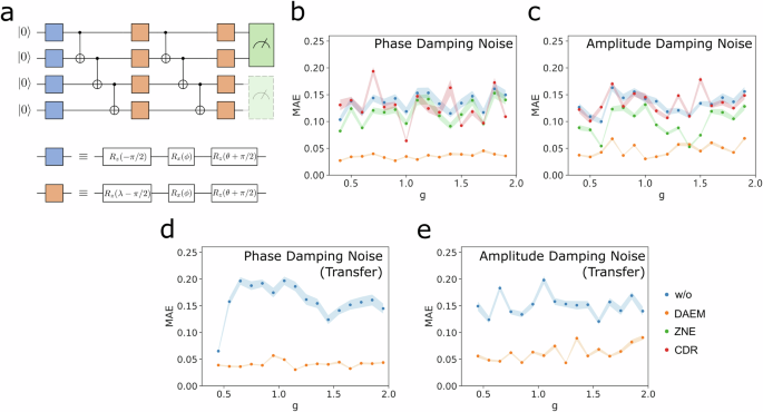
a The variational ansatz for preparing the ground states of 4-qubit transverse Ising models. b Mean Absolute Errors (MAE) between the mitigated measurement expectation values for phase damping noise model and ideal expectation values. c Mean Absolute Errors (MAE) between the mitigated measurement expectation values for amplitude damping noise model and ideal expectation values. d Mean Absolute Errors (MAE) between the mitigated measurement expectation values for phase damping noise model and ideal expectation values for the circuits not included in the training. e Mean Absolute Errors (MAE) between the mitigated measurement expectation values for amplitude damping noise model and ideal expectation values for the circuits not included in the training. It is noteworthy that ZNE requires knowledge of noise parameters associated with statistics while our proposed DAEM not. Despite being under an unfair comparison, DAEM still demonstrates superior performance.

Full size image

During the Error-Mitigation phase, we evaluate our mitigation model by using the prepared initial state ({rho }_{0}=leftvert 0rightrangle {leftlangle 0rightvert }^{otimes N}).

First, we evaluate our model’s performance under two Markovian noise models: amplitude damping and phase damping. In all of the experiments, noise is applied after each gate in Fig. 2a. The amplitude damping noise channel and the phase damping noise channel are mathematically defined by Equation (3) and Equation (6), respectively. Throughout all of our experiments, we consider a set of noise parameters denoted as ({{{lambda }_{k}}}_{k = 1}^{K}in [0.05,0.29]), with stride 0.02.

with ({V}_{0}=left[begin{array}{cc}1&0\ 0&sqrt{1-lambda }end{array}right]) and ({V}_{1}=left[begin{array}{cc}0&sqrt{lambda }\ 0&0end{array}right]). Figure 2b illustrates the mitigation results obtained using various error mitigation techniques for VQE circuits affected by phase damping noise, while Fig. 2c presents the mitigation results for VQE circuits affected by amplitude damping noise. The results clearly demonstrate that DAEM consistently outperforms other mitigation methods for each VQE circuit, regardless of the specific value of g.

Furthermore, we tested our trained model on circuits for preparing ground states of the Ising model with parameters not included in the training set, using the same variational ansatz. Specifically, we varied the parameter g within the range of [0.45, 1.95] with a stride of 0.1. We present the experimental results for mitigating phase damping noise and amplitude damping noise in Fig. 2d, e. The results demonstrate that our model can efficiently transfer error mitigation knowledge to circuits sharing the same ansatz but with different parameters, without requiring further training.

In addition to the Markovian noise model, we also investigate the impact of Non-Markovian noise, which, despite its relevance in real-world quantum experiments^45,46,47, has received limited attention in previous error mitigation studies. Specifically, we consider the multi-qubit spin-boson model⁴⁸ for phase damping to exemplify this scenario, in which a quantum system interacts with the environment, namely, a heat bath, and evolves jointly. This is a potential noise happening in superconducting quantum circuits⁴⁹. In this setup, depicted in Fig. 3a, the system Hamiltonian H_S corresponds to the VQE circuit, while the heat bath is modeled as a bosonic system. We assume each gate in the circuit interacts independently with a bath attached locally. The bath Hamiltonian is ({H}_{B}={sum }_{k}{omega }_{k}{b}_{k}^{dagger }{b}_{k}). Here b_k is the annihilation operator for mode k, and ω_k is the corresponding energy. The interaction between the system and the bath is captured by the Hamiltonian ({H}_{SB}={sum }_{k}{sigma }_{z}otimes [{lambda }_{k}{b}_{k}+{lambda }_{k}^{* }{b}_{k}^{dagger }]), where σ_z is Pauli-Z operator, and ({lambda }_{k}propto 1/sqrt{{omega }_{k}}). We initiate the system and bath as a product state state ρ₀ ⊗ ρ_B, where ρ₀ is the initial state of the system, namely (leftvert 0rightrangle leftlangle 0rightvert). The bath ({rho }_{B}={e}^{-beta {H}_{B}}/Z) is a Gibbs state, with β = 1/(k_BT) and Z being a normalization factor. The evolution of the system under noisy conditions is represented as ({rho }_{S}(t)={{rm{Tr}}}_{B}(U(t)({rho }_{0}otimes {rho }_{B}){U}^{dagger }(t))). Here, (U(t)=exp [-imathop{int}nolimits_{0}^{t}H(tau )dtau]) is the unitary describing the joint evolution of the whole system, with H = H_S + H_B + H_SB. Importantly, it should be noted that this noise is gate-dependent, as gate parameters rely on the evolution time of the Hamiltonians, leading to varying noise effects.

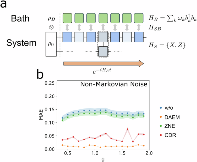
a Schematic diagram of quantum circuits affected by Non-Markovian noise. b Mean Absolute Errors (MAE) between the mitigated measurement expectation values for considered Non-Markovian noise model and ideal expectation values.

Full size image

To modulate this noise, we vary the Hamiltonian evolution time within the range of [0.05, 0.3], while maintaining the computational impact constant.The numerical results, as depicted in Fig. 3b, consistently demonstrate the remarkable effectiveness of our model in handling Non-Markovian noise scenarios. This performance is particularly significant because Non-Markovian noise, a common occurrence in practical quantum experiments^45,46,47, poses a substantial challenge for error mitigation techniques. The robustness of our model in such conditions significantly enhances its practical utility and reliability in the realm of quantum computing.

To further illustrate the effectiveness of our model in practical scenarios, we tested its performance on the real quantum computing hardware provided by OriginQ Cloud⁵⁰. Based on the types of gates available on this hardware, we adopted the variational ansatz shown in Fig. 4a. The circuit is composed of three layers of U₃ gates and two layers of controlled-Z gates. We selected 10 circuits, varying the parameter g within the range of [1.0, 2.0) with a stride of 0.1. The choices of J, N, ({mathcal{M}}), and ({mathcal{S}}) were kept consistent with those used in the simulation experiments above. During the Noise-Awareness phase, we construct the fiducial circuit by replacing each U₃ gate with two U₃ gates that cancel each other out under noiseless conditions, while keeping the CZ gates unchanged, as shown in Fig. 4b.

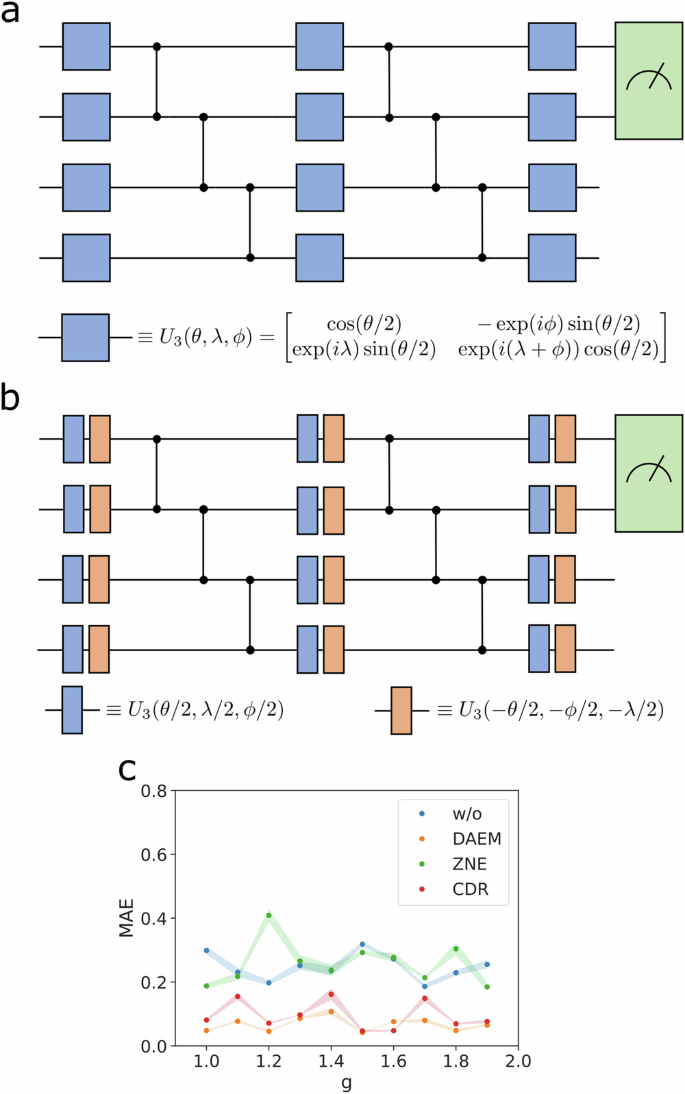
a The variational ansatz for preparing the ground states of 4-qubit transverse Ising models. b The structure of fiducial circuits. c Mean Absolute Errors (MAE) between the mitigated measurement expectation values and ideal expectation values. The average MAE of w/o, DAEM, ZNE, CDR are 0.247, 0.067, 0.259, and 0.095 respectively.

Full size image

Given the difficulty of adjusting noise strength in real experiments, we consider only one noise level (K = 1) for our model. As the results shown in Fig. 4c, our DAEM model demonstrates superior performance in most cases compared to CDR. Note that ZNE cannot be applied in this scenario directly as it requires measurement data from circuits with varying noise strengths. For comparison, we used the method of unitary folding⁵¹ to generate data with four different noise levels for ZNE. Although our model uses data from fewer noise levels than ZNE, it still achieves significant advantages over ZNE.

Swap test

The swap test is a technique used to measure the dissimilarity between two quantum states. In Fig. 5a, we illustrate the circuit designed for comparing two 5-qubit states. When executed on the quantum device, the CSWAP gate is implemented by decomposing it into three Toffoli gates, which are further decomposed using Hadamard, S, T, and CNOT gates. The details are provided in “Methods” section. The circuit takes two input quantum states, (leftvert psi rightrangle) and (leftvert phi rightrangle), for comparison. It initializes the first control qubit as (leftvert 0rightrangle) and produces expectation value that equals the fidelity between two pure states, i.e., ∣〈ψ∣ϕ〉∣², by performing a Pauli Z measurement on the first control qubit. Here, we assume that noise takes place before each controlled-SWAP gate. Specifically, we examine phase damping channel, which can be characterized by the following equation:

with ({V}_{0}=left[begin{array}{cc}1&0\ 0&{e}^{-2lambda }end{array}right]) and ({V}_{1}=left[begin{array}{cc}0&0\ 0&sqrt{1-{e}^{-4lambda }}end{array}right]). λ represents the scale of the noise and P_i are three Pauli gates. We use a set of noise parameters denoted as ({{{lambda }_{k}}}_{k = 1}^{K}={0.05,0.08,0.12,0.15}) in this experiment.

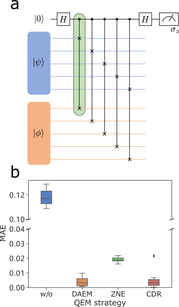
a The swap test circuit for comparing two 5-qubit states. The gate within the green box is the controlled-SWAP gate. b Mean Absolute Errors (MAE) between the mitigated fidelity values and the ground truth values.

Full size image

In the Noise-Awareness phase, the controlled-SWAP gates in Fig. 5 are first decomposed into single-qubit and CNOT gates. ({{mathcal{N}}}_{lambda }({mathcal{F}})) is constructed by replacing all single-qubit gates by two gates that cancel each other. Specifically, for a quantum gate G, we replace it by (sqrt{{G}^{dagger }}sqrt{G}). We randomly select n input states ({{{sigma }_{{s}_{1}}}}_{{s}_{1} = 1}^{n}), where each ({sigma }_{{s}_{1}}=leftvert psi rightrangle leftlangle psi rightvert otimes {sigma }_{{s}_{1}}^{1}otimes {sigma }_{{s}_{1}}^{2}), with (leftvert psi rightrangle) being a random 1-qubit pure state, and ({sigma }_{{s}_{1}}^{1}) and ({sigma }_{{s}_{1}}^{2}) representing two random 5-qubit product states.

In the Error-Mitigation phase, we evaluate our model using 20 pairs of input states ρ₁, ρ₂ in the swap test circuit. We collect statistics by conducting Pauli Z measurements on the first qubit within the noisy swap test circuit. These measurements are subsequently used to compute the overlap between ρ₁ and ρ₂. The noisy expectation values obtained from these measurements are then input into the trained neural model, which produces mitigated values as output. In Fig. 5b, we present Mean Absolute Errors (MAE) between the mitigated values and the ground truth values, providing a comparative analysis with two other quantum error mitigation techniques, ZNE and CDR. The performance of DAEM stands out, showcasing significant improvements over ZNE and demonstrating comparable performance with CDR.

Quantum approximate optimization algorithms

QAOA⁵² is a quantum algorithm specifically designed for solving combinatorial optimization problems. The core of this algorithm involves encoding the objective function of the target optimization problem into a Hamiltonian, and trains an elaborately designed parameterized circuit to approximate the ground state. The final solution is derived by sampling bitstrings from the circuit’s output in the computational basis. However, when running a well-trained QAOA circuit on noisy quantum computers, the resulting output distribution deviates from the ideal scenario, which results in less accurate solutions. Hence, our goal is to mitigate this noise-induced bias in the output distribution, thereby providing experimenters with more precise solutions.

In this specific application, we focus on implementing QAOA for the maximum cut (Max-cut) problem⁵³. The goal is to find a bi-partition of graph G, namely subsets A and B, in which the partition contains the maximum number of edges. This can be defined as an optimization with objective

where i, j denote the indices of vertices, (i, j) represents the edge connecting vertex i and vertex j, and E is the set containing all edges of the graph. If vertex i belongs to subset A, then z_j = 1, otherwise z_j = 0. We provide an instance of G with six vertices in Fig. 6a. The corresponding Hamiltonian of this problem in QAOA can be described by the following:

where Z is Pauli-Z operator. The circuit for QAOA, shown in Fig. 6b, typically comprises two sets of parameterized quantum gates, alternating between a mixing operator ({H}_{B}=mathop{sum }nolimits_{n = 1}^{N}{sigma }_{n}^{x}) and the problem-specific cost operator H_C. In the Noise-awareness phase, to generate fiducial process, after replacing all single-qubit gates with identity gates, the CNOT gates automatically cancel each other. In this case, the fiducial process is trivially identity ideally, i.e., ({{mathcal{N}}}_{0}({mathcal{F}})=I). Again, we execute the fiducial process on noisy quantum devices with different noise parameters to acquire noisy bitstring distributions. Besides, we sample input states (leftvert psi rightrangle) in computational basis to obtain labels for training. In Fig. 6c, we present the mitigated results concerning the output state of a trained QAOA circuit applied to the graph depicted in Fig. 6a. Here, we consider the depolarizing noise model and it can be described by

where P_i are the 4^N − 1 Pauli gates excluding the identity gate. It’s evident that the mitigated frequency of measurement results closely approximates the ideal scenario, signifying that we can obtain more reliable solutions to the original Max-Cut problem through our DAEM model. It’s worth noting that both ZNE and CDR are designed specifically for mitigating errors in expectation values, and they cannot be applied directly to the probability distribution of measurement results, in contrast to our proposed DAEM.

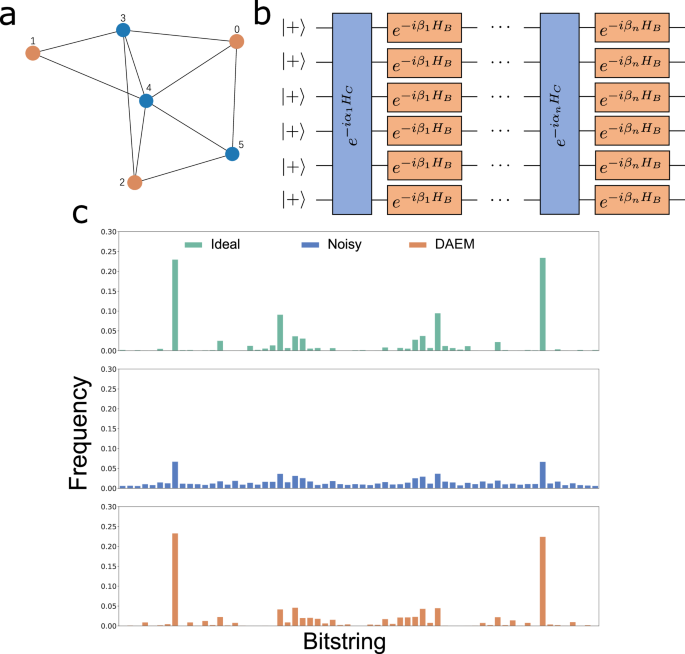
a An instance of a graph for the Max-cut problem. b The variational ansatz for implementing QAOA algorithm. c Ideal, Noisy, and Mitigated frequency of measurement results.

Full size image

Error mitigation for many-body dynamics

Our model works for quantum processes beyond the circuit model. It applies to, for example, the dynamics of physical systems. In this section, we delve into the challenge of error mitigation within the domain of many-body dynamics, which is fundamental to various applications in quantum physics and materials science.

Here, our focus is on the dynamics of a 50-qubit quantum system with an Ising Hamiltonian H_Ising, described in Eq. (1). We consider the whole system’s evolution for time t, given as (U=exp (-{i}{H}_{{rm{Ising}}}t)). This specific process is characterized by the following parameters: J = 1, g = 2, and a time duration of t = 5. For the initial states involved in this Ising Hamiltonian evolution, we have selected the ground states of the Ising model, varying J within the range [−2, 2], while keeping g constant at 1. To simulate these processes, we employ a combination of two powerful techniques: the density matrix renormalization group (DMRG)⁵⁴ and time-evolving block decimation (TEBD)^55,56. In this setup, noise is introduced after the completion of the unitary quantum process. Specifically, we evaluate our model’s performance under two distinct noise models: phase damping and amplitude damping channels. For the set of measurements ({mathcal{M}}), we also consider all two-qubit Pauli measurements on nearest-neighbor qubits. The results, corresponding to different values of g in the input states, are presented in Fig. 7. We can observe that both our model and ZNE have achieved nearly perfect mitigation, as evidenced by the MAE between the mitigated expectation values and the ground-truth values, which are close to zero. We conjecture the reason for the nearly perfect performance of ZNE in this experiment is that no SPAM errors have been introduced. This makes the actual measurement expectation values decay quadratically with respect to the noise parameters, perfectly fitting the ansatz of ZNE. It is important to highlight that ZNE relies on precise knowledge of the noise parameters corresponding to the noisy measurement data, whereas our DAEM model does not have this requirement. CDR is a technique tailored for quantum circuits, and therefore, it cannot be employed to mitigate errors in spin-system dynamics.

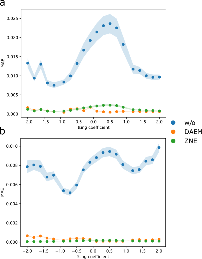
a Mean Absolute Errors (MAE) between the mitigated measurement expectation values for phase damping noise model and ideal expectation values. b Mean Absolute Errors (MAE) between the mitigated measurement expectation values for amplitude damping noise model and ideal expectation values.

Full size image

Error mitigation for continuous-variable processes

Continuous-variable quantum systems have demonstrated their potential in diverse applications including quantum cryptography⁵⁷ and quantum computing⁵⁸. However, despite the growing significance of this type of system, no prior research has discussed the issue of error mitigation within continuous-variable quantum systems as far as we know. In this section, we applied our proposed DAEM model to address this long-unexplored challenge first.

We assess the effectiveness of our method on the dynamics induced by Kerr’s nonlinear interaction⁴³, which is important for continuous variable quantum computing⁵⁸. Consider a quantum system initially prepared in a coherent state (leftvert alpha rightrangle) and subjected to the Kerr Hamiltonian ({H}_{{rm{kerr}}}=pi {hat{a}}^{dagger 2}{hat{a}}^{2}), where (hat{a}) and ({hat{a}}^{dagger }) represent the annihilation and creation operators. In this scenario, we model the noisy process by a lossy open system, whose dynamics are described by the Lindblad master equation:

Here, ({mathcal{D}}(hat{a})(rho ):= hat{a}rho {hat{a}}^{dagger }-frac{1}{2}(rho {hat{a}}^{dagger }hat{a}+{hat{a}}^{dagger }hat{a}rho )), and λ represents the loss rate. Our objective is to mitigate the errors in this process, making it closely resemble the ideal closed-system dynamics governed by Schrödinger’s equation with Hamiltonian H_kerr. In this setting, we consider the measurement results associated with the point-wise Wigner function^59,60. In our numerical experiments, we initialize the state as coherent state (leftvert alpha rightrangle) with α = 1.5 and dimension N = 15. We vary the evolution time over the interval t ∈ [0, 1], considering different loss rates λ ∈ {0.6, 0.65, 0.7, 0.75, 0.8}. To train the neural model within DAEM, we construct the fiducial process ({{mathcal{N}}}_{lambda }({mathcal{F}})) by implementing the evolution of two inverse Hamiltonians, ensuring that the overall effect on the input state is an identity operation under noiseless conditions. Specifically, assuming a total evolution time of t₀, the state evolves with the Hamiltonian H_kerr for t ≤ t₀/2, and with –H_kerr for t₀/2 ≤ t ≤ t₀. We assess the effectiveness of our DAEM by computing the fidelities between the mitigated states and their noiseless counterparts, employing the values of the point-wise Wigner function. As shown in the numerical results presented in Fig. 8a, the fidelity between the state affected by the noise and the ideal state decreases rapidly as time increases. In contrast, our method excels in mitigating this effect, resulting in a dramatic improvement in fidelity. We also present snapshots of the state at different time points in Fig. 8b, and our mitigated point-wise measurement results are notably closer to the ideal ones, particularly for longer evolution.

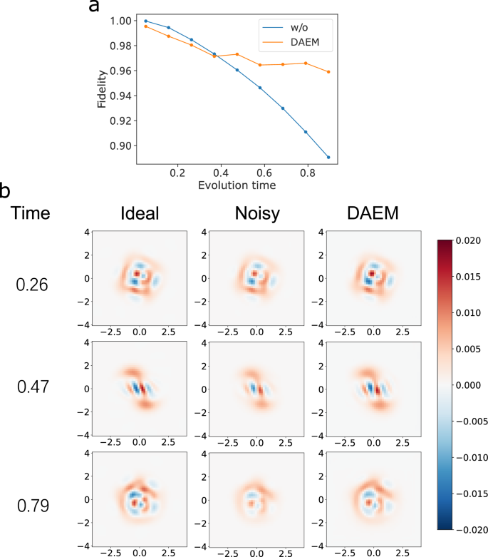
a Fidelity values between the noisy/mitigated state and the ideal output state. b Snapshots of the point-wise measurement results of the state at different time points.

Full size image

The workhorse of our model is the quantum data augmentation method, which generates the training data by letting the unknown noise act on a set of ideal fiducial processes. This technique is not only applicable to quantum error mitigation, but also to other tasks in quantum information processing, including in particular the task of enhancing parameter estimation in quantum metrology⁶¹. By combining quantum data augmentation with the representational capability of deep neural networks, our model becomes able to effectively handle complex noise scenarios. For example, it deals effectively with Non-Markovian noise (viz. Fig. 2e), for which other neural models, like ZNE, tend to perform poorly due to reliance on a predefined extrapolation algorithm.

Our model also offers appealing features compared to conventional error mitigation methods. In CDR, an error mitigation model is better trained with classically simulated quantum circuits that resemble the target circuit⁷. Therefore, the effectiveness of CDR can depend heavily on how closely the training circuits match the target circuit, and achieving such a close match might not always be feasible in practical experiments. In contrast, our proposed DAEM model conducts training directly on the data collected from the hardware, targeting the specific noise to be mitigated. This approach ensures more accurate and effective error mitigation tailored to the actual noise characteristics of the hardware. It is also worth observing that CDR and ZNE are effective at mitigating expectation values, but generally less effective at mitigating the whole probability distribution of the measurement outcomes, a task that is necessary in quantum algorithms like QAOA. For noise preservation, our approach shares a similar spirit with ref. ³⁶, which targets mitigating errors in QAOA circuits. Reference ³⁶ works by considering a modified version of the original circuit, where all single-qubit R_Z gates in the cost gates are ignored. This corresponds to a modified problem Hamiltonian whose ZZ coupling strength is zero, and thus the modified circuit can be simulated efficiently with a classical computer. The modified circuit is then executed on a (noisy) quantum computer. As the (pairwise) CNOT gates are left unchanged in the modified circuits, the outputs of the real-device execution can be compared with the simulation to learn the pattern of noise propagation. Likewise in our framework, we elaborately design our data augmentation strategy that preserves the skeletons of the circuits. Our approach can also be compared to probabilistic error cancellation^2,11,12, which estimates noise-free expectation values by representing them as linear combinations of expectation values from a set of noisy quantum circuits. To work out the appropriate decomposition, this method requires a tomography of the noise, thus resulting in an overhead in sample complexity. A benefit of our approach is that it removes the need for tomography and replaces it with the quantum data augmentation procedure, which is generally less demanding in terms of number of measurement settings.

In terms of scalability, our model can potentially be scaled to larger systems. We conduct experiments on mitigating errors of circuits with different number of qubits and different circuit depth, with a fixed number of training data. Results show that our model can keep stable performance with respect to different circuit configurations. Further information can be found in Supplementary Note 4.

Finally, our model has the potential for extension to mitigate a broader range of realistic quantum errors, including crosstalk errors^62,63, which are common in quantum computing systems. Crosstalk errors result from hardware imperfections that violate the assumption of locality and independence of quantum operations, and are therefore challenging to model⁶⁴. Despite these challenges, error mitigation for crosstalk errors could become approachable in our framework, which does not require prior error modeling.

Neural model in DAEM

Our error mitigation is model-agnostic thus the structure of the neural model can be flexibly chosen, ranging from simple linear models⁶⁵, multi-layer perceptrons (MLP)⁶⁶, to deep neural networks like convolutional neural networks⁶⁷ and Transformers⁶⁸. In practice, we adopt a problem-aware strategy to design the specific construction of the model. In general, we prefer non-linear models for they have stronger ability to capture the intrinsic characteristics of various noise models.

For error mitigation in quantum algorithms and many-body dynamics, we use MLP as the architecture of the neural model. The neural network is composed of multiple layers of fully connected neurons. Each neuron involves one linear transform followed by one non-linear activation. The stack of neurons allows for complex non-linear function fitting, which is powerful for estimating the expectation values and probability distributions in our error mitigation settings. The model’s inputs are parameters indicating the target circuit for mitigation, the observable to be measured, and the measurement statistics. The model’s output is either a real number or a probability distribution obtained by passing through a softmax function, depending on the measurement statistics to be mitigated. The cost function for mitigating expectation values is L₂ loss, namely

where y denotes the output of the neural model and y_fid are the observable expectation values generated from data augmentation using the fiducial channel. The cost function for mitigating probability distribution is the average relative entropy⁶⁹, defined as

where p are probability distribution predicted by our model, and p_fid are distribution obtained from fiducial channel by sampling 10000 shots.

To mitigate errors in continuous-variable processes, we adopt U-Net⁷⁰, a convolutional neural network originally designed for image segmentation⁷¹, to be the neural model denoising the 2-dimensional Wigner function. U-Net possesses the strong ability to extract spatial features and construct 2-dimensional distributions. In this sense, it helps learn the distribution of the point-wise Wigner function. The inputs to the model are evolution time and Wigner functions corresponding to different photon loss rates. The output is a single 2-dimensional feature map, which represents the denoised Wigner function. To train the neural model, we use L₁ loss as cost function, defined as

It encourages sparse output distribution, which conforms to the Wigner quasiprobability distribution of our target states. More details can be found in Supplementary Note 1.

Data augmentation strategy

In practice, the noise-free labels are not available unless we know the exact noiseless output states of the circuits. However, if the input and output states are the same, or under known transformation in the noise-free scenario, we can directly measure the input states to generate labels. Here, we introduce a fiducial process, i.e., ({{mathcal{N}}}_{lambda }({mathcal{F}})), to achieve this goal. The process is trivially identity or contains only CNOT gates that can be absorbed into observables in the noise-free conditions, but share similar noise pattern as the target process in a noisy quantum device. To generate the training set for Noise-Awareness phase, we send input states through the fiducial process, measure the noisy outputs as data and measure the original input states as labels. Note that the input states can be either noisy or noiseless.

We detail the choice of input states and specification of ({{mathcal{N}}}_{lambda }({mathcal{F}})) for different applications as follows.

For swap test circuits, the states to be compared are pure. We decompose the CSWAP gates into three Toffoli gates. The Toffoli gates are further transformed into CNOT and single qubit gates, as shown in Fig. 9.

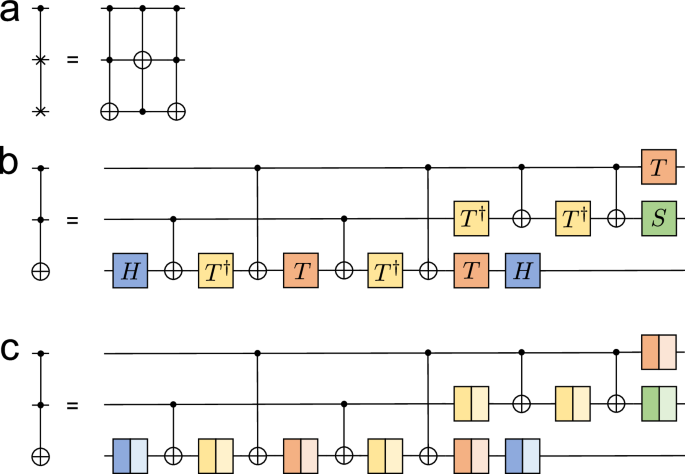
a CSWAP gate is decomposed into 3 Toffoli gates. b Further decomposition of Toffoli gate into single-qubit and CNOT gates. c The corresponding fiducial circuit for training.

Full size image

In Noise-Awarenes phase, we sample 170 random pairs of pure states from the single-qubit Haar measure, in which 100 are used for training, 50 for validation, and 20 for Error-Mitigation phase. For ancilla, we choose random single-qubit mixed states. We construct the fiducial process by replacing every single-qubit gate G with identity gate, which is implemented by (sqrt{{G}^{dagger }}sqrt{G}), leaving the CNOT gates unchanged. This results in a channel ({{mathcal{N}}}_{0}({mathcal{F}})=U), in which U describes the effects of all CNOT gates in the original circuit. Then we execute the fiducial process in noisy environment with varying noise parameters, and measure the noisy outputs using observable M = Z₁, which denotes the Pauli-Z observable on the ancilla qubit, and calculate the expectation values. Meanwhile, we measure the input states with observable (tilde{M}={U}^{dagger }{Z}_{1}U). The measurement expectation values are the corresponding labels.

In VQEs, the augmentation strategy is generally the same as in Swap test. One difference is that, rather than pure states, we randomly sample 100 states as inputs in the Noise-Awareness phase. Whereas in the Error-Mitigation phase, the input states are chosen to be ground state (leftvert 0rightrangle).

For QAOA circuits, note that the distributions of output bitstrings possess symmetry, e.g., if 00011 is one solution, 11100 should also be a solution. To boost the performance of the neural model, we want to make the output distributions of the dataset in Noise-Awareness phase more aligned with those in the Error-Mitigation phase, i.e., the output distributions in the training set also possess this symmetry. It can be mathematically described as ({X}^{otimes n}leftvert psi rightrangle =leftvert psi rightrangle), where X is Pauli-X operator. This shows that the input states (leftvert psi rightrangle) are the eigenvectors of X^⊗n with eigenvalue 1. In our implementation, we sample 100 vectors from the eigenspace of X^⊗n with eigenvalue 1 as the input states. In the Noise-awareness phase, to generate a fiducial process, after replacing all single-qubit gates with identity gates, the CNOT gates automatically cancel each other. In this case, the fiducial process is trivially identity ideally, i.e., ({{mathcal{N}}}_{0}({mathcal{F}})=I). Again, we execute the fiducial process on noisy quantum devices with different noise parameters to acquire noisy bitstring distributions. Besides, we sample input states (leftvert psi rightrangle) in computational basis to obtain labels for training.

For spin systems, the input states in both Noise-Awareness phase and Error-Mitigation phase are sampled from the same distribution. We have 100 different states for training in the first phase and 20 for testing in the second phase. The fiducial process is constructed by simply setting H_Ising = I.

For continuous-variable processes, to generate initial states, we first record intermediate states during noisy evolution of H_kerr in the time interval t ∈ [0, 1], each with a timestep 0.05. With this procedure, we obtain 20 noisy states. Next, for each state, we evolve it with fiducial process ({{mathcal{N}}}_{0}({mathcal{F}})=I) under different loss rates. The fiducial process is generated by H_kerr followed by − H_kerr, which can be simulated on hardware by ref. ⁷². The evolution times of the states are uniformly chosen in the range [0, 1] with a gap of 0.1.

After the completion of this work, another work⁷³ appeared where a data generation technique is employed to mitigate errors in the transverse field Ising model. This approach can be viewed as a specific means of obtaining the fiducial process.