Optimizing bus charging infrastructure by incorporating private car charging demands and uncertain solar photovoltaic generation

Reducing carbon emissions is one of humans’ most critical challenges due to the increasing environmental problems caused by greenhouse gas emissions. The International Energy Agency (IEA) predicts that transportation will become the largest carbon dioxide (CO₂)-emitting sector in the world by 2050¹. Consequently, the transportation sector faces the formidable challenge of reducing CO₂ emissions. Integrating transportation with clean energy is a potential solution to address this challenge. The low-carbon transition of public transportation networks has recently resulted in a sharp rise in electric buses (EBs)². EBs are highly praised for their seamless operation, effective energy conversion, and zero greenhouse gas emissions. In China, public transportation electrification has rapidly expanded, accompanied by the accumulation of extensive operational data and the development of charging infrastructure. As of September 2022, the proportion of clean energy EBs in Beijing had reached 91.7%, and more than 1000 charging stations had been constructed³. In Yinchuan, renewable energy buses comprise 1814 of the 2624 buses or 69.13% of the fleet⁴.

Distributed solar photovoltaic (PV) power generation has become a major renewable energy source in urban areas^5,6, offering notable advantages such as carbon emission savings and reduced energy vulnerability. With advancements in solar PV technology and energy storage, there is a growing interest in integrating solar PV into transportation. As EBs are increasingly adopted, integrating solar PV with EBs provides a way to integrate solar PV into transportation infrastructure, which is vital in promoting carbon reduction^7,8. However, solar PV outputs are uncertain and highly susceptible to stochastic weather conditions, such as solar irradiance availability and temperature variations, which can affect grid stability⁹. Although battery energy storage (BES) has emerged as an effective solution to enhance solar PV utilization and mitigate grid impacts¹⁰, declining battery costs over the past decade, they remain relatively expensive compared to the solar PV system¹¹. Thus, in PV-battery integrated systems, optimizing battery capacities is essential to improve performance while maintaining cost-effectiveness.

Meanwhile, the rapid rise in private electric vehicles (EVs) is driving a noticeable increase in charging demand¹². Urban EV charging infrastructure faces challenges such as the low vehicle-pile ratio and the unbalance between charging supply and demand¹³. Bus charging stations possess advantages for serving private EVs’ charging demands. During off-peak hours, the bus charging facilities are often underutilized, presenting an opportunity to enhance resource utilization through sharing charging services with EVs. Bus charging stations are generally equipped with sufficient high-power chargers, and their dispersed locations throughout the city make them ideal for complementing EV charging networks. Offering shared charging services at bus depots provides economic benefits for public transportation agencies through additional revenue from electricity and service fees. Furthermore, integrating PV and BES systems at shared bus depots could improve PV utilization and lower peak electricity demand from the power grid. In this context, this study proposes a shared bus charging hub that integrates PV and BES. We investigate the optimal deployment of solar PV and BES in this shared hub, accounting for the uncertainty of solar PV generation. The economic, environmental, and grid benefits of integrating shared bus charging infrastructure with solar PV and BES at the bus depot are thoroughly analyzed in Yinchuan, China. In addition, we analyzed several countries to validate the global applicability of integrating solar PV and BES at shared bus depots (Fig. 1).

The framework demonstrates the use of multi-source datasets to estimate the energy supply and demand for bus charging infrastructure. The framework maximizes the economic benefits of bus charging infrastructure with solar PV and BES by optimizing the PV installed capacity, BES capacity, and charger configuration. The framework evaluates the economic, environmental, and grid advantages of bus charging infrastructure during its lifetime.

Full size image

Extensive studies have focused on integrating solar PV power with EV charging infrastructure. Research has shown that integrating solar PV and BES with EV charging stations can lower charging costs, reduce carbon emissions, and alleviate grid loads^14,15,16. Previous works have explored optimal solar PV and BES configurations at charging stations. Huang et al. (2019) developed a genetic algorithm to optimize the placement and capacity of solar PV panels in a hybrid system incorporating heat pumps and thermal storage¹⁷. Their case study demonstrated that the integrated system effectively increased the self-consumption rate of solar PV power at the district level to about 77%. Wu et al. (2022) analyzed household energy demand, proposing an allocation method for optimal household energy costs, considering variable EV charging patterns and BES degradation¹⁸. The findings suggested that BES could effectively reduce household peak power demand, indicating that integrating PV, BES, and EVs is the most cost-effective solution for individual households. Several studies have also examined vehicle charging strategies alongside capacity planning for solar PV and BES in EV charging infrastructure. Liu et al. (2020) considered a coordinated charging strategy for EVs when planning solar PV and BES capacity and validated the advantages of the approach¹⁹. The proposed optimization model minimized the energy purchase costs, solar PV and BES investment costs, and maintenance costs of the fast charging station. Dong et al. (2024) incorporated charging scheduling optimization in the capacity planning model for solar PV and BES-integrated EV charging stations, and they proposed a hybrid modeling approach for solar PV²⁰. The study confirmed the effectiveness of the method by using a typical commercial region as a research scenario. The results showed a 15.67% improvement in economic benefits and a 37.14% reduction in carbon emissions compared to grid-based charging.

In the past four years, research has expanded to include electric buses (EBs) within this framework. Liu et al. (2024) explored transforming bus stations into energy hubs using data from over 200 million GPS records from nearly 21,000 buses in Beijing²¹. The results indicated that converting bus depots into renewable energy hubs can generate economic gains and CO₂ savings while reducing the grid charging load of battery EBs. Dalala et al. (2020) examined the economic and environmental benefits of integrating solar PV above bus parking and routes in the Amman Bus Rapid Transit Project, finding positive results from measures such as installing elevated PV panels and using LED lighting²². In addition, previous studies focused on examining vehicle charging and energy scheduling when integrating distributed solar PV and BES with EBs, illustrating the economic and environmental benefits of the integration system^23,24,25. Besides research on the possibilities and advantages of integrating solar PV and BES with EBs, several optimization methods for implementing solar PV and BES at bus depots have also been documented in previous studies. To find the optimal configuration of solar PV and BES in bus charging stations, Liu et al. (2023) employed a surrogate-based optimization approach²⁶. They used data from Beijing, China to study the benefits of integrating solar PV and BES into EB charging stations, showing the reduction of the total cost of charging and CO₂ emissions after introducing these systems. Ren et al. (2022) devised an integer linear programming model solved by a genetic algorithm to determine the optimal solar PV and BES for bus depots¹⁶. The model considered the costs and the benefits of solar PV and BES to minimize the payback period. They constructed a real-world case study in Hong Kong to demonstrate the effectiveness of the optimal deployment.

However, current research has not addressed the economic, environmental, and grid impacts of integrating solar PV and BES with EBs in scenarios where bus depots are shared with private EVs. Most existing studies have utilized model-driven methods to analyze integrated charging infrastructure. Although these methods enable the optimization and regulation of energy and transit systems, their heavy reliance on assumptions often results in solutions that are not practical in real-world scenarios. Furthermore, a few studies do not consider the uncertainty in solar PV generation, which can lead to suboptimal performance under real-world conditions²⁷, as actual PV power outputs may differ from those assumed during the design phase^28,29.

This study addresses existing gaps with the following contributions. We propose a novel solution that integrates bus charging infrastructure with solar PV and BES while accommodating private EVs with available chargers. A comprehensive analysis of the economic, environmental, and grid impacts is conducted using real-world case studies. We adopt a data-driven approach, leveraging a multi-source dataset to estimate solar PV generation, electric bus consumption, and EV charging demand distribution. We incorporate the seasonality and uncertainty of solar PV generation into capacity planning to enhance the robustness and resilience of the proposed solutions.

Solar PV power outputs

The solar PV power generation scenarios derived from the Latin Hypercube Sampling (LHS) method are shown in Fig. 2. In this study, we sample the solar PV power generation data every month and use the k-means clustering method to cluster the monthly sampled data into three scenarios representing three typical climatic conditions. Figure 2 illustrates the solar PV power generation results for each typical climate for the four seasons of spring, summer, autumn, and winter, respectively. For example, Fig. 2c shows the solar PV power generation results in autumn, where typical scenario 1 corresponds to a climate characterized by high solar PV power generation, while typical scenarios 2 and 3 indicate relatively low power generation.

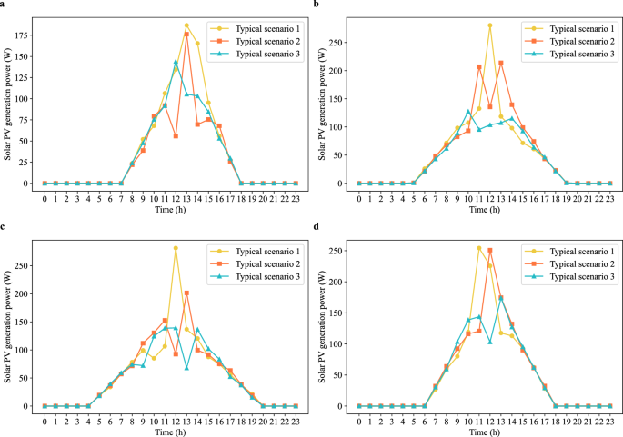
a Daily solar PV power generation in spring. b Daily solar PV power generation in summer. c Daily solar PV power generation in autumn. d Daily solar PV power generation in winter.

Full size image

EB energy consumption

The estimation results indicate that the average energy consumption per kilometer is 1.23 kWh, closely aligning with established research findings³⁰. To reveal the seasonal impacts on the EB energy consumption, we utilize a real energy consumption dataset from 2019, which includes data from 56 electric buses in Beijing, comprising over 210,000 records of energy consumption and charging sessions³¹. We select May as a baseline month in Yinchuan and calculate the adjustment coefficients for the other months relative to May, as shown in Table 1. Based on the adjustment coefficients, we estimate the energy consumption for the remaining months. The daily total energy consumption for EBs across different months is illustrated in Fig. 3.

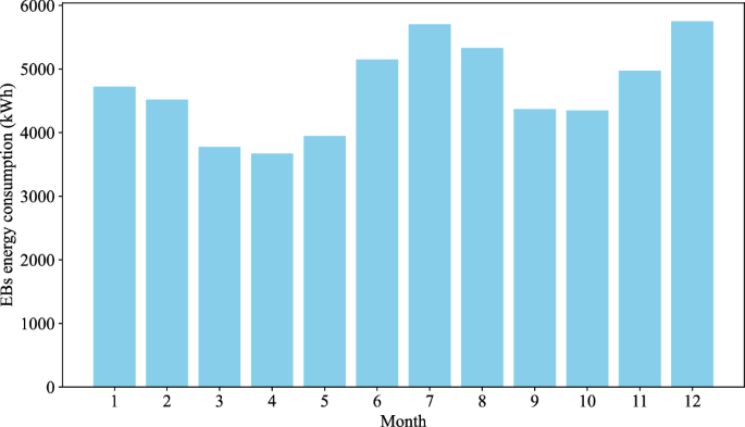
This figure shows the daily energy consumption of EBs across different months. Each month, there are differences in energy consumption due to various factors such as air temperature, and we analyze each month to show the seasonal differences in EB energy consumption.

Full size image

EV charging demand

To estimate the demand for EV charging near bus depots in Yinchuan, we first determine the EV penetration rate to be 3.99%. This calculation is based on a total of 1,324,100 motor vehicles in the city³², of which 52,808 are EVs³³. Additionally, there are 1,158,400 private vehicles and 1,126,200 households in Yinchuan³⁴, leading to an average of approximately 1.03 private cars per household. To address the demand for EV charging services, Yinchuan has implemented a “3-kilometer charging service area” measure, which ensures private vehicles are charged within three kilometers of a residential area³³. We estimate that around 3528 households reside within the charging service area of this bus depot³². Combining the average number of private cars per household with the EV penetration rate, we calculate approximately 145 private EV users around the bus depot. According to EV charging reports, one EV user typically charges the EV an average of 0.18 times per day³⁴, with the average charged electricity of 25.2 kWh once³⁵. The total EV charging demand around the bus depot is approximately 656 kWh daily. Based on the EV charging load distribution curve from the existing official report³⁴, we assess the charging demand for private EVs around the bus depot throughout the day, as depicted in Fig. 4. This finding aligns closely with results from the previous study³⁶.

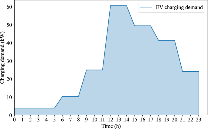
Charging demand for EVs varies with the time of day, peaking at 12:00 to 14:00 and dropping to a minimum in the early morning hours.

Full size image

Infrastructure configuration at the bus depot

The optimal capacity of BES is determined to be 11.75 kWh. This capacity is sufficient to store excess solar energy or purchase electricity when electricity prices are low, allowing BES to provide power for bus charging during periods of low solar generation or when electricity prices are high. To meet both the bus charging demand and the BES storage requirements, the bus depot is equipped with 1840 solar PV panels. Additionally, the depot deploys 6 chargers, each with a maximum charging power of 358 kW. The number of chargers is primarily determined by the number of buses parked at the depot simultaneously, ensuring that all buses can be charged without delays. Due to the relatively small number of chargers, the charging power is optimized to be as high as possible to enable fast charging.

Economic, environmental, and grid impacts of bus charging hubs

We compare the model results with and without solar PV and BES to evaluate the economic and environmental benefits. In the baseline scenario, where solar PV and BES are not integrated, EBs are charged solely using grid electricity with a First-In, First-Out principle. Our findings show that the proposed optimization model with solar PV and BES reduces total costs by 37.35% over the 10-year lifetime of BES despite the higher construction costs associated with solar PV and BES. Additionally, integrating private EVs into the bus depot can generate an annual revenue of 5502 USD for public transportation agencies, showcasing potential economic benefits. Notably, this economic benefit comes from the charging service fee and price gap between electricity price and solar PV utilization.

From an environmental perspective, the integration of solar PV and BES results in a 41.47% reduction in carbon emissions over the 10-year period, demonstrating the environmental advantages of integrating solar PV and BES into bus charging infrastructure. To assess the environmental impact of the battery production process, we use data from the European Organization for Clean Transportation and Energy. Their estimates suggest that the carbon footprint of producing a typical lithium-ion battery in China is 105 kg CO₂e/kWh³⁷. Based on this, the carbon emissions associated with manufacturing the 11.75 kWh energy storage battery used in this study would amount to 1234.14 kg. When accounting for the carbon emissions from battery production, the overall reduction in carbon emissions from the charging facility incorporating both solar PV and BES is 41.46%. Given the relatively low capacity of BES, its impact on total carbon emissions is minimal.

We select representative regions and countries for analysis to further validate the benefits of integrating solar PV and BES at shared bus depots globally. The data regarding solar PV costs and carbon pricing are sourced from the report by the IEA³⁸, while energy storage costs are derived from the IEA’s “Batteries and Secure Energy Transitions” report³⁹. Additionally, regional electricity pricing information is gathered through an open-source dataset⁴⁰. To assess the impact of economic factors, such as installation costs and electricity prices, we standardize the bus charging demand across all regions and calculate the optimal results for different countries, allowing for an equitable comparison of the economic and environmental outcomes under varying local conditions. The findings, illustrated in Fig. 5, indicate that this integration strategy can result in varying economic cost reductions: 8.43%in the United States, 36.21% in the European Union, and 16.69% in Australia. In addition, carbon emissions in these countries and regions are reduced by 22.81% in the United States, 27.44%% in the European Union, and 35.39% in Australia. Overall, this research emphasizes the potential of integrating renewable energy solutions to enhance sustainability in public transportation systems worldwide. Supplementary Table 1 shows the key parameters in the optimal deployment model for different regions and countries. Supplementary Table 2 provides the optimal infrastructure deployments for these regions and countries.

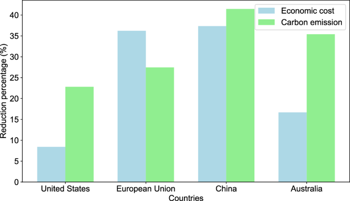
The figure illustrates the percentage reductions in both economic costs and carbon emissions across four regions: the United States, the European Union, China, and Australia. The blue bar indicates economic cost, and the green bar indicates carbon emission. These data highlight the economic and environmental benefits of combining solar PV and BES at the bus charging hub in each country and demonstrate the regional differences in the economic and environmental benefits of sustainable energy practices.

Full size image

Figure 6 presents the charging load at the bus depot under different scenarios: the bus depot without private EV access and solar PV integration, the bus depot with integrated solar PV and BES, and the shared bus depot with integrated solar PV and BES. As shown in Fig. 6, the integration of solar PV and BES shifts the majority of the EB charging load to midday, when solar radiation is strongest, thereby reducing the peak charging demand typically seen around 17:00. Although the introduction of private EV charging increases the overall load, the load distribution still largely aligns with peak solar radiation periods. This demonstrates a clear correlation between vehicle charging behavior and renewable energy generation from solar PV.

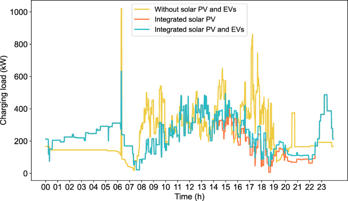
We show the hourly charging load over a day, comparing three scenarios: without solar PV and EVs, with integrated solar PV, and with both solar PV and EV integration. The yellow line represents the scenario without solar PV and EVs, which demonstrates the highest peaks and variability. The orange line, depicting integrated solar PV, shows reduced peak loads and smoother fluctuations. The blue line shows the charging load with both solar PV and EV integration.

Full size image

Additionally, integrating solar PV and BES into a shared bus charging hub reduces the overall grid load to a 49.35% reduction in net charging loads. It significantly alleviates stress on the grid over the 10-year lifetime of BES. To better visualize the impact of shared bus charging depot on grid demand, Fig. 7 compares the grid load of a bus depot with EV charging but without solar PV integration to the grid load of a shared bus charging hub that incorporates both solar PV and BES. The results clearly demonstrate that the integration of solar PV and BES effectively lowers the grid load. During periods of high solar PV generation, the energy produced can fully meet the charging demand of both EBs and private EVs, thereby reducing dependence on the grid and further decreasing grid load during peak periods.

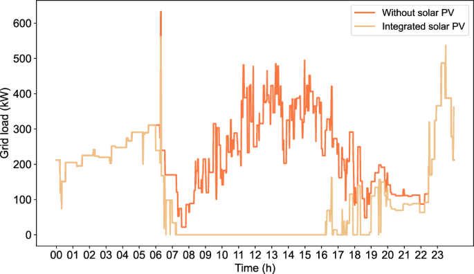
We show the grid load over a day, comparing scenarios without and with solar PV integration. The orange line represents grid load without solar PV, showing higher peaks, particularly around noon and early afternoon. The beige line, indicating grid load with integrated solar PV, demonstrates significant reductions during peak times and overall smoother load fluctuations.

Full size image

Sensitivity analysis of model parameters

The sensitivity analysis evaluates the impact of parameters on the solutions generated by the model. Specifically, this analysis focuses on the construction price per unit for BES and solar PV, as well as the electricity sales price of solar PV. To assess the influence of these parameters, we use the values listed in Table 2 as a baseline and vary them within a range of 50% to 150%.

We first explore the effect of the construction price of BES on the solutions generated by the model. Figure 8 illustrates the change in the model results as the construction price of BES increases. The x-axis denotes the ratio of the construction price of BES to the original value in Table 2, while the y-axis denotes the ratio of the optimal results to the original one. From Fig. 8a, it can be seen that with the construction price of BES increasing, the total costs shift from −0.94% to 0.14%. The optimization results of decision variables with different construction prices of BES are compared in Fig. 8b. As depicted in Fig. 8b, the capacity of BES rapidly decreases as the construction price increases, attributable to its incorporation into the model’s objective function. Additionally, the findings indicate that the quantities of PV panels and chargers remain unaffected by the BES price. Comparing Fig. 8a and Fig. 8b, we observe that while the construction price of BES notably influences its capacity, its impact on the total costs is relatively minor. This is attributed to the model’s results indicating a small BES capacity, consequently resulting in minimal cost implications.

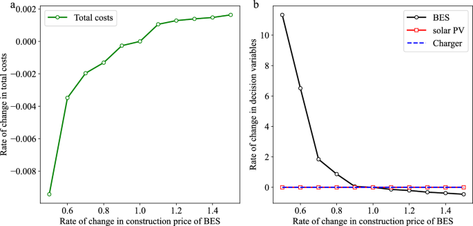
a The change in the total costs as the construction price of BES increases. b The change in the decision variables as the construction price of BES increases.

Full size image

The analysis further examines the impact of the construction price of solar PV on the model’s outcomes. Figure 9 illustrates the fluctuations in the optimal results with respect to the construction price of solar PV. As shown in Fig. 9a, as the construction price of solar PV increases, the total costs shift from −10% to 10%. Figure 9b presents the optimization results of decision variables under different construction prices of solar PV. The results indicate that the construction price of solar PV does not affect these variables. Consequently, it only impacts the total costs, leading to linear variations corresponding to the unit cost.

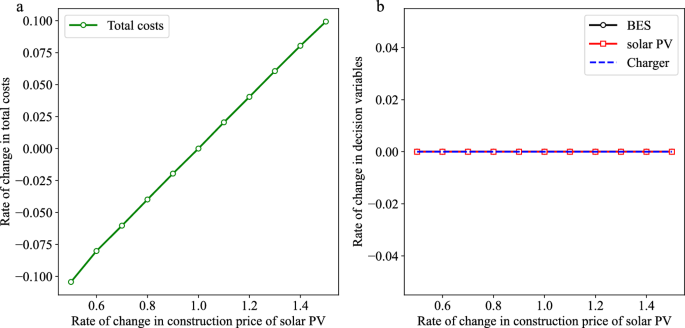
a The change in the total costs as the construction price of solar PV increases. b The change in the decision variables as the construction price of solar PV increases.

Full size image

To comprehend the impacts of fluctuating solar PV electricity sales prices on optimal outcomes, Fig. 10 investigates how alterations in sales prices of solar PV power influence the total costs and the decision variables. The findings reveal that as the sales price of solar PV power rises from 50% to 150%, the total costs fluctuate from 9.03% to −14.53%, whereas the capacity of BES fluctuates from 50.17% to −87.68%. When the sales price of solar PV power surpasses the original value outlined in Table 2, the BES capacity experiences a rapid decline. This phenomenon occurs because the lower sales price of solar PV power has little effect on the BES capacity, while the system prioritizes selling surplus solar PV energy over storing it in BES at higher prices, leading to a rapid reduction in total costs.

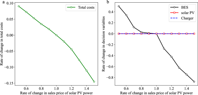
a The change in the total costs as the sales price of solar PV power increases. b The change in the decision variables as the sales price of solar PV power increases.

Full size image

The sensitivity analysis shows that the number of chargers deployed at bus depots remains unaffected. Furthermore, the construction price of solar PV does not influence the number of PV panels, as the economic benefits of building the solar PV system outweigh its costs, highlighting the advantages of integrating solar PV with bus charging infrastructure.

A data-driven approach to optimize solar photovoltaic-based bus charging infrastructure under uncertain power outputs is proposed in this study to achieve economic, grid, and environmental benefits. The optimal strategy considers the charging events of all buses at the bus depot and the availability of chargers. Realistic constraints related to battery energy storage and power conservation of the integrating system are applied. It is novel that we consider the uncertainty of solar photovoltaic generation and propose an operational scenario that opens the bus depot to private electric vehicles to satisfy their charging demand and generate revenue for public transportation agencies.

To validate the effectiveness of the optimization model, a typical scenario of a bus depot in Yinchuan, China, is constructed using multi-source heterogeneous data such as bus trajectory, depot, and smart card data. The results indicate that the proposed optimization model can decrease costs by 37.35% and carbon emissions by 41.46% over the 10-year lifetime of storage batteries compared to the selected bus depot without solar photovoltaic and battery energy storage, which relies on grid-based infrastructure. Additionally, integrating private electric vehicles into the bus depot can generate an annual revenue of 5502 USD, indicating the potential economic benefits of social networking operations at the bus depot. The integrated system also reduces grid charging loads by 49.35%, alleviating grid stress. In contrast to an existing study that focuses on electrifying entire bus networks in cities such as Beijing²¹, our approach focuses on optimizing a single bus depot that operates as an energy hub. This site-specific analysis shows that solar PV can effectively meet the charging demands of electric vehicles at the bus depot, resulting in enhanced economic, environmental, and grid advantages. Furthermore, this study explores the applicability of integrating solar PV and BES at bus depots in various countries, revealing different economic and environmental benefits. This broader analysis validates the global relevance of the proposed approach. A sensitivity analysis is employed to examine how model parameters affect the solutions. The results reveal that the construction prices of solar photovoltaic and battery energy storage influence the total costs. Notably, the construction price of solar PV does not affect the number of solar PV panels, suggesting that the economic advantages of integrating solar PV with the bus charging infrastructure outweigh its costs.

The proposed approach shows promise for achieving an optimal capacity configuration of integrated bus charging infrastructure with solar photovoltaic and battery energy storage. However, the current model needs to incorporate rich electric bus charging strategies for different charging technologies (e.g., fast charging, slow charging, and Panto Down chargers). Future research will also focus on integrating the various energy management measures (e.g., smart charging) and scheduling optimization methods to enhance the realism of the results.

Dataset

To evaluate the performance of the developed optimization model, we use a comprehensive dataset to conduct a case study in Yinchuan, China. This dataset includes the geographical coordinates of a representative bus depot where 45 EBs operate in a continuous cycle. Each bus departs from and returns to a single depot for recharging. The dataset also contains high-precision GPS trajectory information, recording details such as time, altitude, longitude, latitude, and velocity of the buses on a particular day in 2019. Additionally, smart card data is also used, which includes information on card ID, stop information, boarding time, and alighting time.

As shown in Table 2, the case study’s parameter settings are described as follows. The construction price of solar PV of 1 kW is 4000 CNY⁴¹, with a life cycle of 25 years⁴² and an aging rate of 0.5% per year⁴³. We assume the resale price of solar PV is 5% of the original cost. The construction price of BES of 1 kWh is 1950 CNY, expected to serve for 10 years⁴⁴. Let the annual capacity degradation rate of BES be 2.5%²¹. Furthermore, the price for a charger with a power rating P is calculated a ({{rm{beta }}}_{1}{rm{P}}+{{rm{beta }}}_{0}), where β₁ and β₀ take values of 0.22 and 12.24, respectively⁴⁵. We assume that the chargers have a lifespan of 10 years. The operational horizon for the optimal deployment method spans one day and is segmented into one-minute intervals. This study measures the daily costs associated with solar PV, BES, and chargers. Regarding environmental costs, the carbon emissions cost associated with electricity generated by coal-fired power plants is 0.0544 CNY per kWh. In comparison, the electricity generated by solar PV systems incurs a lower carbon emissions cost of 0.0054 CNY per kWh²⁶. In addition, a service fee of 0.3 CNY per kWh is applied to private EVs charged at the bus depot⁴⁶. We also consider the excess solar PV power sold to the grid at a rate of 0.2595 CN per kWh⁴⁷. Regarding operational constraints, the minimum SOC permitted for EB and BES is set at 20%. EBs initialize with a 100% SOC, whereas BES begins at a SOC of 50%. We assume the capacity of the EB power battery is 300 kWh. The maximum power of BES is 150 kW, and the charging and discharging efficiency is set at 0.87. Details on utility electricity prices are provided in Table 3. The available roof areas for PV panel deployment at this bus depot, estimated based on remote sensing images, indicate a potential for deploying 4549 PV panels.

Estimation of solar PV power outputs under uncertainty

To estimate the output power of PV panels, two key environmental factors are considered: solar irradiance, represented by (S_m), and ambient temperature, represented by (T_a). The output power (P_m) of a specific PV panel, given its known parameters, can be calculated as follows⁴⁸:

Where T_n represents the working temperature of PV panels, and T_cell represents the working temperature of PV panels. P_r and θ are the rated output power and temperature power coefficient of PV panels, respectively.

The intermittent, stochastic, and fluctuating nature of solar energy poses complex challenges for solar PV power generation⁴⁹. To address the stochastic characteristics inherent in solar PV output, we transform uncertain factors into a series of deterministic scenarios through simulation analyses of potential situations. This study uses the LHS method to sample solar PV power outputs to generate a scenario set. This technique facilitates the sampling of variables such as ambient temperature and solar irradiance, enabling the management of inherent uncertainty in these factors. Consequently, this method provides a robust framework for generating scenarios that effectively capture the stochastic nature of solar PV outputs. The detailed sampling process of LHS is as follows⁵⁰:

Firstly, suppose the sampling size is N, the random variable size is m, the sample space is expressed as (X=left[begin{array}{cc}{X}_{1} & {X}_{2}end{array}cdots {X}_{m}right]), and ({X}_{i}left(i=1,2,cdots ,mright)) is i-th random variable in the sample space X. The cumulative distribution function is expressed as:

Where X_i is the input random variable, and ({{rm{F}}}_{{rm{i}}}left({{rm{X}}}_{{rm{i}}}right)) is its cumulative distribution function. Let P_i denote the sum of all probabilities less than or equal to the value.

Secondly, the curve ({F}_{i}left({X}_{i}right)) is divided into N sections along the longitudinal coordinate axis, [(n-1)/N,n/N], n=1, 2(cdots)N, and each section is evenly spaced and non-overlapping, having a uniform width of 1/N.

Lastly, the midpoint (left(n-0.5right)/N) of each interval is chosen as the sample value of P_i, and the inverse value of Eq. (3) is employed to determine the sample value of X_i. This process yields the n-th sample value of X_i as Eq. (4) shows. When each random variable is sampled by N times, an initial sampling matrix of m × N order can be generated.

To account for the uncertainty of solar PV power generation across different months, we first define the parameter ranges based on monthly variations in solar radiation, angle, and temperature. Using these ranges, we apply the LHS method to generate 100 sets of PV generation parameters for each month. For each of these 100 parameter sets, we use a PV power generation estimation model to calculate the corresponding daily solar PV power outputs. This process results in a collection of 100 daily solar PV generation scenarios for each month, capturing the variability and uncertainty of solar PV power generation throughout the year.

The scenario reduction can reduce the original scenario sets to overcome computational complexity while preserving the integrity of the scenario analysis and retaining typical climate characteristics. Due to its advantage in managing large-scale stochastic optimization challenges with fewer iterations and reduced computational demands, the k-means clustering algorithm is an ideal choice for scenario reduction in this study.

The k-means clustering method uses the Euclidean distance as the similarity criterion, and the expression is:

In Eq. (5), ({S}_{i}=left({x}_{i1,}{x}_{i2},cdots {x}_{{iw}}right)) is an w-dimensional data sample.

After generating multiple scenario samples using LHS based on mathematical modeling of solar PV output power, we apply the k-means clustering technique to reduce the number of scenarios. This process allows us to identify typical scenarios and their associated probabilities. In this study, we clustered the 100 PV power samples generated for each month into three representative scenarios, each corresponding to a typical climate condition for PV power generation. This approach enhances the practical relevance of our results by providing a more informative set of scenarios for analysis.

Estimation of EB energy consumption

This study uses a longitudinal dynamics model for EVs to estimate the energy consumption of EBs⁵¹. Firstly, the traction force can be calculated as follows:

({{rm{F}}}_{{rm{drag}}}={{rm{K}}}_{{rm{d}}}{{rm{v}}}^{2}) is the aerodynamic drag, with ({{rm{K}}}_{{rm{d}}}=0.5{rm{rho }}{{rm{C}}}_{{rm{d}}}{rm{A}}), ρ refers to the air mass density in ({rm{kg}}/{{rm{m}}}^{3}), C_d is the drag coefficient, A is the reference frontal area of the vehicle in m², and v is the vehicle speed in m/s. ({{rm{F}}}_{{rm{roll}}}={rm{Mgf}}cos left({rm{alpha }}right)) is the rolling friction. f is the rolling resistance coefficient. ({{rm{F}}}_{{rm{climb}}}={rm{Mg}}sin left({rm{alpha }}right)) is the slope force. M is the total mass of the vehicle in kg, g is the gravitational acceleration ((9.81{rm{m}}/{{rm{s}}}^{2})), α is the road slope and is calculated by using the elevation difference ∆h and the distance D between two bus stops, such that (tan alpha =triangle h/D). ({{rm{F}}}_{{rm{intertia}}}={rm{delta }}{rm{Ma}}) is the inertia force resulting from the change of kinetic energy stored by the vehicle (acceleration or deceleration), and a is the acceleration of the object. δ is a factor that considers the inertia of all rotating components in the drivetrain (wheels, drives, motor shafts, rotors, etc.). According to the number of passengers in the vehicle, the total mass of the vehicle M can be calculated as the sum of curb weight M_curb and total mass of passengers in the vehicle: ({rm{M}}={{rm{M}}}_{{rm{curb}}}+{{rm{eta }}}_{{rm{pax}}}{{rm{m}}}_{{rm{pax}}}).

Equation (7) can be used to determine the energy consumption produced by traction force during a trip between adjacent stops. In addition, the losses in the motor, inverter, and drivetrain are calculated through the efficiency parameter η.

This study also examines the auxiliary power P_aux required for auxiliary services (such as powered steering, operating doors, etc.) and air conditioning.

Where E_aux is auxiliary energy demand, (triangle {t}_{{trip}}) is the driving duration, and (triangle {t}_{{dwell}}) is the dwell time.

Hence, EB energy consumption is:

Due to restricted data gathering conditions, it is hard to obtain high-resolution measurements for the driving profiles of all buses, which complicates the computation of the integral of Eq. (7). To solve this problem, we effectively estimate bus energy consumption using synthetic driving profiles made from GPS trajectories and smart card data⁵¹.

Estimation of EV energy demand

In this study, we present a hypothetical scenario where bus depots are made accessible to private EVs for charging. A simulation method is employed to estimate EVs’ charging demand in this context. Firstly, the number of charging users in the vicinity of public transportation sites (N_a) is estimated as follows:

Where r is the radius of the charging service area around the bus depot, A is the total area of the administrative region, and H is the total number of households.

Subsequently, the attraction of bus depots to nearby EV charging users (Q) can be calculated by Eq. (11).

Where N_a is the number of charging users in the vicinity of public transportation sites, N_b is the average number of private cars per household, and R is the EV penetration rate.

After determining the average number of charge sessions per household (({{rm{N}}}_{{rm{c}}})) and the charging demand per session (({{rm{D}}}_{{rm{p}}})), the charging demand of a single EV user (({{rm{D}}}_{{rm{s}}})) can be calculated as follows:

The total energy demand of EVs around the bus depots (({rm{D}})) is then given by Eq. (13).

However, to analyze the temporal distribution of charging demand, it is necessary to further disaggregate ({rm{D}}) over time. This is achieved by applying the time distribution of user charging behavior, which reflects the probability of users charging during different periods of the day. This approach allows for a detailed estimation of charging demand across various time intervals.

Mixed integer linear optimization model

As illustrated in Fig. 11, this study focuses on a single bus depot integrated with solar PV and BES. All EBs operate on a cyclical basis, departing from and returning to this depot, where EBs and EVs undergo charging processes utilizing solar PV, BES, and grid electricity. This integrated bus depot serves as an energy hub for charging operations, incorporating solar PV and grid connectivity to efficiently meet charging requirements. The available roof areas for PV panel deployment at the bus depot are estimated based on remote sensing images shown in Fig. 11. Next, our study will address the optimization problem of solar PV capacity, BES capacity, the configuration of chargers, energy management, and charging schedule at bus depots.

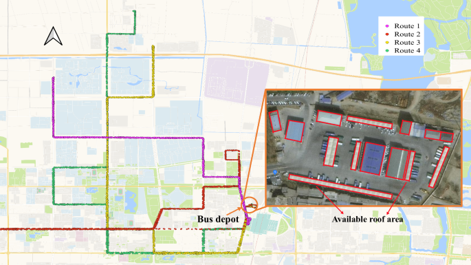
The different colored dots in the figure indicate the GPS track points of the EBs on different routes, showing the trajectories of the EBs. The EB trajectories are grouped together at one point, which is the bus depot. EBs operating four routes are charged at this bus depot, which can use its free roof to install PV modules. This bus depot is an energy hub for charging operations, incorporating solar PV and BES.

Full size image

Let I denote the set of EBs. Let L denote the set of bus layovers. Let Y denote the set of years. Let M denote the set of months in a year. Let K represent the set of solar PV power generation scenarios. This study divides one day into T equal blocks, each representing one minute. Table 4 presents the model concepts of sets, indices, parameters, and decision variables.

Mixed integer linear optimization model objective function

As stated in Eq. (14), the optimization objective is to minimize the sum of the total costs associated with the bus depot over the 10-year lifetime of BES, which includes seven components. The first term measures the costs associated with the integrated charging infrastructure incorporating solar PV and BES. This includes the construction costs of the solar PV, BES, and chargers. The second term accounts for the expense incurred from purchasing electricity from the grid. The third term calculates the costs associated with carbon emissions from the grid and solar PV. The fourth term represents the revenue generated from service fees for providing charging infrastructure to EVs. The fifth term denotes the revenue generated from selling solar PV energy to the grid. The sixth term represents savings in the cost of purchased electricity from the grid. The last term accounts for the residual value of the solar PV modules after 10 years. The objective function can be formulated as follows.

Where ({lambda }_{{bat}},) ({lambda }_{{pv}}) are the unit prices of BES and PV panel. The price of a charger with maximum charging power ({rm{P}}) is represented by ({{rm{beta }}}_{1}{rm{P}}+{{rm{beta }}}_{0}), where ({{rm{beta }}}_{1}) and ({{rm{beta }}}_{0}) are assumptions based on available charger price data⁵². ({{rm{rho }}}_{{rm{y}},{rm{m}},{rm{k}}}) is the probability of solar PV power generation scenario k occurring in month m of year y. ({{rm{d}}}_{{rm{m}}}) is the number of days in month m. Let ({{rm{r}}}_{{rm{BES}}}) denote the annual capacity degradation rate of BES. (triangle t) is a time division, it is set to be one minute in this paper. ({{rm{lambda }}}_{{rm{t}}}) is the unit price of purchasing electricity from the grid in time slot t. ({rm{P}}_{{rm{grid}},{rm{t}}}^{{rm{y}},{rm{m}},{rm{k}}}) and ({rm{P}}_{{rm{pv}},{rm{t}}}^{{rm{y}},{rm{m}},{rm{k}}}) are the charging power for all the vehicles from the grid and the solar PV output power in time slot t under solar PV power generation scenario k in month m of year y. δ_grid and δ_pv are the carbon emission cost of thermal power generation and solar PV power generation. ({rm{N}}_{{rm{ev}},{rm{t}}}^{{rm{y}},{rm{m}},{rm{k}}}) denotes the number of chargers occupied by EVs in time slot t under solar PV power generation scenario k in month m of year y and ({{rm{delta }}}_{{rm{ev}}}) represents the service fee of providing the charging infrastructure to EVs. ({{rm{delta }}}_{{rm{sell}}}) is electricity sales price of solar PV. ({{rm{r}}}_{{rm{PV}}}) is the PV module aging rate per year. ({{rm{mu }}}_{{rm{PV}}}) is the residual value rate of solar PV. Let ({{rm{N}}}_{{rm{ch}}}) indicate the number of chargers, ({{rm{N}}}_{{rm{pv}}}) is the number of PV panels, and ({{rm{C}}}_{{rm{bat}}}) represents the capacity of BES at the bus depot.

Mixed integer linear optimization model constraints

1. (1)

   Constraints related to solar PV generation

   The output power of the PV panels at the bus depot in time slot t under solar PV power generation scenario k in month m of year y can be calculated with Eq. (15). The output power of a single PV panel (({{rm{Q}}}_{{rm{t}}}^{{rm{y}},{rm{m}},{rm{k}}})) is determined based on the solar PV power prediction method previously described.

   $${{rm{P}}}_{{rm{pv}},{rm{t}}}^{{rm{y}},{rm{m}},{rm{k}}}={{rm{N}}}_{{rm{pv}}}{{rm{Q}}}_{{rm{t}}}^{{rm{y}},{rm{m}},{rm{k}}},forall {rm{t}},{rm{epsilon }},{rm{T}},{rm{k}},{rm{epsilon }},{rm{K}},{rm{m}},{rm{epsilon }},{rm{M}},{rm{y}}{rm{epsilon }}{rm{Y}}$$

   (15)
2. (2)

   Constraints related to EB charging

   The charging power for each bus is restricted by the maximum charging power of chargers deployed at the bus depot, shown as Eq. (16). Meanwhile, the EB battery’s SOC is limited to a minimum (({rm{SO}}{{rm{C}}}_{min })) to a maximum (({{rm{SO}}C}_{max })) value. By the end of the day or immediately following the last layover, the bus battery SOC is constrained to be equivalent to the initial SOC. Equation (17) defines these constraints.

   $${{rm{P}}}_{{rm{i}},{rm{l}}}^{{rm{y}},{rm{m}},{rm{k}}}le {rm{P}},forall {rm{i}},{rm{epsilon }},{rm{I}},{rm{l}},{rm{epsilon }},{rm{L}},{rm{k}},{rm{epsilon }},{rm{K}},{rm{m}},{rm{epsilon }},{rm{M}},{rm{y}},{rm{epsilon }},{rm{Y}}$$

   (16)
   $$left{begin{array}{c}{rm{SO}}{{rm{C}}}_{{rm{bef}},{rm{i}},{rm{l}}}^{{rm{y}},{rm{m}},{rm{k}}}ge {rm{SO}}{{rm{C}}}_{min },forall {rm{i}},{rm{epsilon }},{rm{I}},{rm{l}},{rm{epsilon }},{rm{L}},{rm{k}},{rm{epsilon }},{rm{K}},{rm{m}},{rm{epsilon }},{rm{M}},{rm{y}},{rm{epsilon }},{rm{Y}}\ {SO}{C}_{{aft},i,l}^{y,m,k}le {SO}{C}_{max },forall i,{rm{epsilon }},I,l,{rm{epsilon }},L,k,{rm{epsilon }},K,m,{rm{epsilon }},M,y,{rm{epsilon }},Y\ {SO}{C}_{{aft},i,L}^{y,m,k}={SO}{C}_{{ini}},forall i,{rm{epsilon }},I,k,{rm{epsilon }},K,m,{rm{epsilon }},M,y,{rm{epsilon }},Yend{array}right.$$

   (17)

   Where ({rm{P}}_{rm{i}},{rm{l}}^{{rm{y}},{rm{m}},{rm{k}}}) is the charging power for EB i during the layover l under solar PV power generation scenario k in month m of year y. ({rm{SO}}{rm{C}}_{{rm{bef}},{rm{i}},{rm{l}}}^{{rm{y}},{rm{m}},{rm{k}}}) and ({rm{SO}}{rm{C}}_{{rm{aft}},{rm{i}},{rm{l}}}^{{rm{y}},{rm{m}},{rm{k}}}) are the bus battery’s SOC of EB i right before and right after the layover l under solar PV power generation scenario k in month m of year y, respectively. They can be described as follows:

   $${rm{SO}}{{rm{C}}}_{{rm{bef}},{rm{i}},{rm{l}}}^{{rm{y}},{rm{m}},{rm{k}}}={rm{SO}}{{rm{C}}}_{{rm{ini}}}-frac{{{rm{e}}}_{{rm{i}},{rm{l}}}}{{rm{C}}},{rm{l}}=1,forall {rm{i}},{rm{epsilon }},{rm{I}},{rm{k}},{rm{epsilon }},{rm{K}},{rm{m}},{rm{epsilon }},{rm{M}},{rm{y}},{rm{epsilon }},{rm{Y}}$$

   (18)
   $${rm{SO}}{{rm{C}}}_{{rm{bef}},{rm{i}},{rm{l}}}^{{rm{y}},{rm{m}},{rm{k}}}={rm{SO}}{{rm{C}}}_{{rm{aft}},{rm{i}},{rm{l}}-1}^{{rm{y}},{rm{m}},{rm{k}}}-frac{{{rm{e}}}_{{rm{i}},{rm{l}}}}{{rm{C}}},{rm{l}},ne ,1,forall {rm{i}},{rm{epsilon }},{rm{I}},{rm{k}},{rm{epsilon }},{rm{K}},{rm{m}},{rm{epsilon }},{rm{M}},{rm{y}},{rm{epsilon }},{rm{Y}}$$

   (19)
   $${rm{SO}}{{rm{C}}}_{{rm{aft}},{rm{i}},{rm{l}}}^{{rm{y}},{rm{m}},{rm{k}}}={rm{SO}}{{rm{C}}}_{{rm{bef}},{rm{i}},{rm{l}}}^{{rm{y}},{rm{m}},{rm{k}}}+frac{{{rm{P}}}_{{rm{i}},{rm{l}}}^{{rm{y}},{rm{m}},{rm{k}}}{rm{du}}{{rm{r}}}_{{rm{i}},{rm{l}}}}{{rm{C}}},forall {rm{i}},{rm{epsilon }},{rm{I}},{rm{l}},{rm{epsilon }},{rm{L}},{rm{k}},{rm{epsilon }},{rm{K}},{rm{m}},{rm{epsilon }},{rm{M}},{rm{y}},{rm{epsilon }},{rm{Y}}$$

   (20)

   Equation (21) is used to constrain the number of concurrent occupied chargers.

   $${{rm{N}}}_{{rm{bus}},{rm{t}}}^{{rm{y}},{rm{m}},{rm{k}}}le {{rm{N}}}_{{rm{ch}}},forall {rm{t}}{rm{epsilon }}{rm{T}},{rm{k}},{rm{epsilon }},{rm{K}},{rm{m}},{rm{epsilon }},{rm{M}},{rm{y}},{rm{epsilon }},{rm{Y}}$$

   (21)

   Where ({rm{N}}_{{rm{bus}},{rm{t}}}^{{rm{y}},{rm{m}},{rm{k}}}) is the number of occupied chargers in time slot t under solar PV power generation scenario k in month m of year y. It can be evaluated according to the bus charging schedule in Eq. (22). The coefficient matrix derived from the bus schedule is the first term on the right. This matrix has vectors (i.e., ({rm{Sc}})) in each column that represent the length of a charging event. (overline{{P}_{i,l}^{y,m,k}}) is the dummy variable of ({rm{P}}_{rm{i}},{rm{l}}^{{rm{y}},{rm{m}},{rm{k}}}). (overline{{P}_{i,l}^{y,m,k}}) is 1 if ({rm{P}}_{{rm{i}},{rm{l}}}^{{rm{y}},{rm{m}},{rm{k}}}) is larger than zero, otherwise 0.

   $$left[begin{array}{c}{N}_{{bus},1}^{y,m,k}\ {N}_{{bus},2}^{y,m,k}\ vdots \ {N}_{{bus},T}^{y,m,k}end{array}right]=left[begin{array}{cccccc}S{c}_{1,1}^{y,m,k} & cdots & S{c}_{1,L}^{y,m,k} & S{c}_{2,1}^{y,m,k} & cdots & S{c}_{{rm{I}},{rm{L}}}^{y,m,k}end{array}right]left[begin{array}{c}overline{{P}_{1,1}^{y,m,k}}\ vdots \ overline{{P}_{1,L}^{y,m,k}}\ overline{{P}_{2,1}^{y,m,k}}\ vdots \ overline{{P}_{I,L}^{y,m,k}}end{array}right]$$

   (22)
   $${rm{Sc}}_{{rm{i}},{rm{l}}}^{{rm{y}},{rm{m}},{rm{k}}}={left[begin{array}{cccccccccc}0 & cdots & 0 & 1 & 1 & cdots & 1 & 0 & cdots & 0end{array}right]}^{T}$$

   (23)

   For instance, in Eq. (23), if the bus i stops at the bus depot in time slot t under PV power generation scenario k in month m of year y, the value in the matrix (({rm{S}}{{rm{c}}}_{{rm{i}},{rm{l}}}^{{rm{y}},{rm{m}},{rm{k}}})) representing this time slot is set to 1; otherwise, it is set to 0. This method is employed to derive the duration matrix for all buses.

3. (3)

   Constraints related to EV charging

   When private EVs arrive at the bus depot, they can only utilize the available chargers to avoid conflicts in bus charging operations. Moreover, the bus depot is not obligated to accommodate every private EV charging request; instead, it offers this service as an optional provision. These constraints are defined by Eq. (24), Eq. (25), and Eq. (26).

   $${{rm{N}}}_{{rm{ev}},{rm{t}}}^{{rm{y}},{rm{m}},{rm{k}}}le {{rm{N}}}_{{rm{ch}}}-{{rm{N}}}_{{rm{bus}},{rm{t}}}^{{rm{y}},{rm{m}},{rm{k}}},forall {rm{t}},{rm{epsilon }},{rm{T}},{rm{k}},{rm{epsilon }},{rm{K}},{rm{m}},{rm{epsilon }},{rm{M}},{rm{y}},{rm{epsilon }},{rm{Y}}$$

   (24)
   $${{rm{P}}}_{{rm{ev}},{rm{t}}}^{{rm{y}},{rm{m}},{rm{k}}}={rm{P}}{{rm{N}}}_{{rm{ev}},{rm{t}}}^{{rm{y}},{rm{m}},{rm{k}}},forall {rm{t}},{rm{epsilon }},{rm{T}},{rm{k}},{rm{epsilon }},{rm{K}},{rm{m}},{rm{epsilon }},{rm{M}},{rm{y}},{rm{epsilon }},{rm{Y}}$$

   (25)
   $${{rm{P}}}_{{rm{ev}},{rm{t}}}^{{rm{y}},{rm{m}},{rm{k}}}le {{rm{P}}}_{{rm{ev}},{rm{t}}},forall {rm{t}},{rm{epsilon }},{rm{T}},{rm{k}},{rm{epsilon }},{rm{K}},{rm{m}},{rm{epsilon }},{rm{M}},{rm{y}},{rm{epsilon }},{rm{Y}}$$

   (26)
4. (4)

   Constraints related to BES

   The maximum and minimum thresholds (({rm{SO}}{{rm{C}}}_{max},{rm{and}}; {{SO}}{{C}}_{min })) define the boundaries of the SOC of the battery in BES. Additionally, the end-of-day SOC of the battery in BES must be equivalent to its initial SOC.

   $$left{begin{array}{c}{{rm{E}}}_{{rm{bat}},{rm{t}}}^{{rm{y}},{rm{m}},{rm{k}}}le {rm{SO}}{{rm{C}}}_{max }{{rm{C}}}_{{rm{bat}}},forall {rm{t}},{rm{epsilon }},{rm{T}},{rm{k}},{rm{epsilon }},{rm{K}},{rm{m}},{rm{epsilon }},{rm{M}},{rm{y}},{rm{epsilon }},{rm{Y}}\ {E}_{{bat},t}^{y,m,k}ge {SO}{C}_{min }{C}_{{bat}},forall t,{rm{epsilon }},T,k,{rm{epsilon }},K,m,{rm{epsilon }},M,y,{rm{epsilon }},Y\ {E}_{{bat},T}^{y,m,k}={SO}{C}_{{ini}}{C}_{{bat}},forall k,{rm{epsilon }},K,m,{rm{epsilon }},M,y,{rm{epsilon }},Yend{array}right.$$

   (27)

   ({rm{E}}_{{rm{bat}},{rm{t}}}^{{rm{y}},{rm{m}},{rm{k}}}) denotes the energy remaining in BES in time slot t under solar PV power generation scenario k in month m of year y, which can be calculated by Eq. (28) and Eq. (29). ({rm{P}}_{{rm{charge}},{rm{t}}}^{{rm{y}},{rm{m}},{rm{k}}}) and ({rm{P}}_{{rm{discharge}},{rm{t}}}^{{rm{y}},{rm{m}},{rm{k}}}) denote the charging power and the discharging power of BES in time slot t under solar PV power generation scenario k in month m of year y, respectively. Let ({rm{varepsilon }}) represent the charging and discharging efficiency. For the first minute of a day, the energy remaining is calculated by Eq. (29).

   $${{rm{E}}}_{{rm{bat}},{rm{t}}}^{{rm{y}},{rm{m}},{rm{k}}}={{rm{E}}}_{{rm{bat}},{rm{t}}-1}^{{rm{y}},{rm{m}},{rm{k}}}+,{rm{varepsilon }},triangle {rm{t}}{{rm{P}}}_{{rm{charge}},{rm{t}}}^{{rm{y}},{rm{m}},{rm{k}}}-frac{triangle {rm{t}}{{rm{P}}}_{{rm{discharge}},{rm{t}}}^{{rm{y}},{rm{m}},{rm{k}}}}{{rm{varepsilon }}},{rm{t}},ne ,1,forall {rm{k}},{rm{epsilon }},{rm{K}},{rm{m}},{rm{epsilon }},{rm{M}},{rm{y}},{rm{epsilon }},{rm{Y}}$$

   (28)
   $${{rm{E}}}_{{rm{bat}},{rm{t}}}^{{rm{y}},{rm{m}},{rm{k}}}={rm{SO}}{{rm{C}}}_{{rm{ini}}}{{rm{C}}}_{{rm{bat}}}+,{rm{varepsilon }},triangle {rm{t}}{{rm{P}}}_{{rm{charge}},{rm{t}}}^{{rm{y}},{rm{m}},{rm{k}}}-frac{triangle {rm{t}}{{rm{P}}}_{{rm{discharge}},{rm{t}}}^{{rm{y}},{rm{m}},{rm{k}}}},{{rm{varepsilon }}},,{rm{t}}=1,forall {rm{k}},{rm{epsilon }},{rm{K}},{rm{m}},{rm{epsilon }},{rm{M}},{rm{y}},{rm{epsilon }},{rm{Y}}$$

   (29)

   Additionally, Eq. (30) and Eq. (31) regulate the simultaneous charging and discharging of BES, where ({q}_{t}^{y,m,k}) is an auxiliary binary variable, and ({rm{Z}}) represents a sufficient large number.

   $${{rm{P}}}_{{rm{charge}},{rm{t}}}^{{rm{y}},{rm{m}},{rm{k}}}{rm{Z}}{{{q}}}_{{{t}}}^{{{y}},{{m}},{{k}}},forall {rm{t}},{rm{epsilon }},{rm{T}},{rm{k}},{rm{epsilon }},{rm{K}},{rm{m}},{rm{epsilon }},{rm{M}},{rm{y}},{rm{epsilon }},{rm{Y}}$$

   (30)
   $${{rm{P}}}_{{rm{discharge}},{rm{t}}}^{{rm{y}},{rm{m}},{rm{k}}}le {rm{Z}}left(1-{{{q}}}_{{{t}}}^{{{y}},{{m}},{rm{k}}}right),forall {rm{t}},{rm{epsilon }},{rm{T}},{rm{k}},{rm{epsilon }},{rm{K}},{rm{m}},{rm{epsilon }},{rm{M}},{rm{y}},{rm{epsilon }},{rm{Y}}$$

   (31)

   The maximum and minimum power requirements for BES operation are introduced in Eq. (32).

   $$left{begin{array}{l}0le {P}_{{charge},t}^{y,m,k}le {P}_{max }\ 0le {P}_{{discharge},t}^{y,m,k}le {P}_{max }end{array}right.,forall {rm{t}},{rm{epsilon }},{rm{T}},{rm{k}},{rm{epsilon }},{rm{K}},{rm{m}},{rm{epsilon }},{rm{M}},{rm{y}},{rm{epsilon }},{rm{Y}}$$

   (32)
5. (5)

   Power conservation constraint

At any given time point, the input power of the system must match the output power. Input power includes power generated by solar PV, purchased from the grid, and discharged from BES. Output power equals the sum of power sold back to the grid and charging power for EBs, private EVs and BES. Thus, the balance constraint of the system is described as: