Parallel circuit implementation of variational quantum algorithms

Introduction
In recent years the field of quantum computing has grown in terms of interest due to its promise of being able to solve certain problems asymptotically faster than the best-known classical algorithms1,2. Unlike classical computers, quantum computers are analog devices that exploit some properties of quantum mechanics to execute algorithms with improved complexity cost or efficiency. Various theoretical studies demonstrate that such an improvement can be reached and in some cases that the current classical algorithms cannot match this performance1,2,3,4.
Although the promises, at the time of writing, due to the presence of noise which causes errors during the computation, it is not possible to execute such algorithms on quantum hardware (also known as noisy intermediate-scale quantum processors, or NISQ5). Consequently, over the past few years, various algorithms have been developed, known as variational quantum algorithms (VQAs), specifically designed to operate on such small imperfect quantum machines6. These algorithms fall under the class of hybrid quantum-classical algorithms, where a quantum circuit is implemented as a black-box function optimized using a classical method. Typically, circuits are characterized by a set of continuous real parameters in one and two-qubit gates whose values are determined by a classical optimizer—these are said to be parameterized quantum circuits. The goal is to find a set of parameters such that the output of the parameterized quantum circuit minimizes a given objective function. These algorithms present shallow and small circuits that, due to the reduced number of operations, are in general more resilient against noise6.
Despite the challenges presented by state-of-the-art hardware, efforts are being made to make quantum computing practical and applicable to industrial problems. One promising application of quantum computing is to solve hard optimization problems and the sub-field devoted to this is called quantum optimization. Several algorithms were developed in the past with the aim of solving industrially relevant optimization problems7,8.
Current state-of-the-art quantum optimization algorithms require the input problem to be encoded in a formulation, the Quadratic Unconstrained Binary Optimization (QUBO) problem. The goal of a QUBO problem is to find a binary vector (xin {{mathbb{B}}}^{n}) such that the value xTQx is minimized, where Q is a symmetric real matrix9,10. This problem is equivalent to the Ising model, which is a physical model that can be interchanged with QUBOs as input of a quantum algorithm. In the Ising model, the variables are spins that can take values of either +1 or -1 and are encoded in a symmetric matrix similar to QUBOs. A change of basis gives the equivalence between these two models. In various applications of quantum optimization, these models have been demonstrated to be appropriate for representing various combinatorial optimization problems9.
One of the algorithms that uses the Ising Hamiltonian to construct the parameterized quantum circuit is the Quantum Approximate Optimization Algorithm (QAOA) inspired by the adiabatic theorem11. Here, alternating parameterized layers of gates approximate an adiabatic evolution. The solutions obtained are, therefore, approximations of ground states of a given Ising Hamiltonian. The hyperparameters of the quantum circuit are optimized classically in an outer loop by minimizing the average energy of the Ising Hamiltonian evaluated with the samples collected from the QAOA quantum circuit. Hence the QAOA circuit acts as a black-box sampler in the inner loop. There are well-known theoretical results for both finite-depth and infinite-depth circuits which show how QAOA can be used to solve some well-known optimization problems8,12,13,14,15,16. Additional variants of QAOA have been developed in recent years to improve the performance of the algorithm under different optimization conditions (such as error mitigation, feasibility of solutions, etc.)17,18,19,20. A more general VQA approach to optimization is the Variational Quantum Eigensolver (VQE). Here, a quantum circuit is constructed given a problem-independent parameterized ansatz. Then, similarly to QAOA, the parameters of the ansatz are optimized with respect to a given Hamiltonian which represents some quantum system. In literature, VQE has been used to solve the minimum eigenvalue problem, which is equivalent to minimizing an Ising Hamiltonian representation of a combinatorial optimization problem, but can also be used to find ground states of other quantum systems21.
There are, however, significant limitations to the implementation of VQAs in state-of-the-art quantum hardware. The most relevant limiting factor is the number of qubits required to construct the circuits. Although minimizing an Ising Hamiltonian is NP-hard22 and can be used to represent many combinatorial optimization problems of academic and practical interest, this often includes a polynomial overhead in the scaling of resources required to represent such problems9. Typically, the limits of computability for hard problems are well beyond those that can be solved with existing quantum hardware, and so only small toy instances of said problems are typically solved with VQAs. Furthermore, due to high error rates and low coherence times, especially at large depths, the effect of noise becomes non-negligible and reduces the performance of VQAs23. It is important to note that the quality of the results of these VQAs depends on the optimization of the parameters in the quantum circuit by definition. Furthermore, it has been shown that training these parameters optimally is in itself an NP-hard problem24, and as such, implying that finding optimal VQA parameters is at least as hard as solving the combinatorial optimization problems themselves.
Particularly for QAOA variants25 the proposed modifications always aim to exclusively boost the performance rather than address scalability or implementation limitations. In this algorithms, QAOA varies the initial state20 or the layer implementation26,27, increases the number of hyperparameters13, uses post-processing rule to reduce the problem size28. However, in the proposed variants, the required number of qubits and circuit depth scale as in the original proposal. Thus, limiting their implementation. Furthermore, the performance improvement usually comes with a classical overhead in the computational time.
In this work, we present a framework to parallelize any VQA. By applying this framework to VQAs, we can improve the result by maximizing the usage of the limited number of qubits and making the circuit implementation shallower. For the sake of simplicity, we motivate our method using quantum optimization algorithms in particular, although our framework is generalizable to any variational quantum algorithm. The essence of the framework is that we approximate the output of the quantum circuit of the VQA with a Cartesian product of outputs of smaller quantum circuits. In other words, given a combinatorial optimization problem and a VQA quantum circuit, we approximate the ground state distribution of the problem by splitting the ansatz into independent smaller parameterized quantum circuits, each of which is optimized in parallel and guided by a single global objective function. Thus, we exploit the properties of the VQA to find a collection of classically separable quantum systems with shallow circuits whose product of vector spaces matches the original search space of the problem.
Results
An open research question of practical relevance in quantum optimization researchers is how to efficiently implement constrained optimization problems in quantum computers. In general, implementing constraints requires an overhead of resources in terms of qubits and interactions between them9. Therefore, the implementation of larger constrained problems becomes impractical because the number of qubits (and the respective circuit size) is insufficient to meet the requirements of such problems. Hence, while encoding a constraint, we have to minimize the number of additional quantum resources required to implement it. Along this direction, in29,30 possible solutions are presented. The authors proposed not to include the constraint as part of the Hamiltonian that defines the circuit, but rather implement it as part of the function used to optimize the hyperparameters. This results in transferring the information regarding the feasibility of the constraints from the quantum circuit to the classical search (e.g., the “outer loop” component of VQAs), showing some improvement in the quality of the solutions. Additional work in this direction using VQE employs the concept of contextual subspaces in molecular simulations, where a quantum Hamiltonian is split into two separable Hamiltonians, whose sum reconstructs the original Hamiltonian of interest31. One of these Hamiltonians is then computed classically, and the second attempts to “correct” the classical approximation using a VQE method. The number of qubits required to implement such a hybrid method was significantly smaller compared to other VQE methods, while still maintaining the chemical accuracy of the model.
Another viable approach to handle the overhead of qubits and gates while implementing constraints is to apply circuit cutting and knitting techniques30,32. Although these methods show that we can simulate larger quantum systems using fewer qubits and achieve improved solution quality in certain scenarios, this outcome involves a trade-off. Indeed, in both cases the authors highlight that there is an exponential overhead in the number of measurements we have to apply in order to reconstruct the correct wavefunction30 or in the number of cuts we can apply to the circuit, resulting in an exponential search to find the best and suitable way of cutting the circuit32.
Inspired by the techniques presented above, we try to overcome some of the issues and we formalize a framework that approximates any variational quantum algorithm by splitting its quantum part and allowing parallelization.
Parallelizing variational quantum algorithms
We formally define a VQA as a parameterized quantum circuit, with parameters optimized over a real-valued function f. The circuit is initialized with an initial set of parameters and after its execution, the circuit is measured. The samples obtained from the measurements are used to evaluate f and compute a new set of parameters for the following iteration. Then, the classical optimizer updates the parameters and collects new samples. This procedure is repeated until convergence or a desired result is reached.
Due to the scarce resources available in the state-of-the-art quantum hardware, implementing large-sized problems can often be impractical. Our proposed approach tackles this issue by creating several smaller parameterized quantum circuits tailored to the VQA that can be executed on the available resources and whose samples can be used to produce samples of the original circuit of the VQA— we call this approach slicing. The general slicing procedure can be described as follows: consider the parameterized quantum circuit of a VQA defined on N qubits and a quantum register with n qubits upon which we want to implement our quantum circuit. By inspecting the problem, we identify r different subproblems that can be implemented as parameterized quantum circuits— we call the parameterized quantum circuits that implement the subproblems slices. Notice that each slice must be implementable on at most n qubits. The sum of the number of qubits used to implement the slices must equal N. Notice that the outer classical optimization routine is no longer optimizing a black box defined on a 2N-dimensional space, but r black boxes defined on spaces of dimension at most 2n.
The easiest to slice a VQA can be realized by identifying and removing a set of gates that connect classically separable quantum circuits from the parameterized quantum circuit. These gates can be found using well-developed circuit cutting and knitting techniques. However, as we explain in the following section, by examining additional properties of the problem, we can exploit the VQA structure to find tailored parameterized quantum circuits without directly inspecting the circuit.
Given the above framework, we can, specifically, formalize the resulting parallel implementation of the parameterized quantum circuit as the following function
where ({{mathbb{R}}}^{q}) is the search space of the parameters and ({mathbb{U}}({2}^{N})) is the space of unitary matrices of dimension 2N. Therefore, the function ({mathcal{C}}) fulfills:
where ({U}_{i}:{{mathbb{R}}}^{q}longrightarrow mathop{bigcup }nolimits_{j = 1}^{n}{mathbb{U}}({2}^{j})) for all i = 1, …, r.
As we can see from eq. (1), we can represent the circuit described by the unitary matrix ({mathcal{C}}({alpha }_{1},ldots ,{alpha }_{q})) as a tensor product of the classically separable circuits described by the unitary matrices Ui(α1, …, αq). To distinguish between them, we call the samples collected from the circuit represented by ({mathcal{C}}) global samples and the samples collected from the circuit represented by Ui slice samples.
Since ({mathcal{C}}) is a tensor product of unitaries, we can obtain the global samples by computing the tensor product of the slice samples. Thus, if (leftvert {s}_{i}rightrangle) is a slice sample collected from the circuit represented by Ui, the global samples take the form
If each qubit is measured individually, we can see the state (leftvert {s}_{1}{s}_{2}cdots {s}_{r}rightrangle) collected from the quantum circuit as a bit-string. Thus, we can interpret the tensor product (leftvert {s}_{1}rightrangle otimes leftvert {s}_{2}rightrangle otimes cdots otimes leftvert {s}_{r}rightrangle) as a Cartesian product of the bit-strings s1, …, sr. Therefore, we can define the global samples by considering the Cartesian product of the slice samples considered as bit-strings. Let V1, …, Vr be the sets obtained by collecting the slice samples seen as bit-strings from the circuits represented by the unitaries Ui(α1, …, αq). The global samples obtained belong to the set V1 × ⋯ × Vr. The cardinality of this Cartesian product is M1M2 ⋯ Mr, where Mi is the number of slice samples collected from the circuit represented by Ui. Hence, the cardinality of V1 × ⋯ × Vr scales at least exponentially in the number of measurements, i.e. (Theta left({left[mathop{min }limits_{i = 1,ldots ,r}{M}_{i}right]}^{r}right)). Therefore, when the number of slices increases, we must apply a rule to select the global samples from V1 × ⋯ × Vr to make the training of the parameters practical. However, as we show in the next section, if the function f fulfills specific properties, the exponential overhead of samples does not represent a problem for the training of the parameters. Thus, a rule must be applied only when the best solution has to be determined. As an example, in section 4 we present two different rules to obtain the global samples from slice samples.
We can immediately see that, depending on the number of qubits available in the register, we can have different advantages in using our framework. If N > n, implementing the original circuit requires more qubits than the number available in the hardware, therefore the algorithm can only be implemented in its parallelized version. On the other hand, when N ≤ n we can see that even though the circuit can now be implemented, our framework reduces the number of gates used and, therefore, the quantum circuit is shallower. Thus, in both cases, our approach reduces the resources used.
Parallelization of quantum optimization algorithms
In this work, we focus on how to parallelize VQAs to solve combinatorial optimization problems formulated as Ising Hamiltonians. To apply our method, we must define the subproblems to obtain the slices. Thus, we must inspect the Ising Hamiltonian of the given combinatorial optimization problem and find smaller Hamiltonians that represent only part of the problem — these are called slice Hamiltonian, whereas the Hamiltonian that encodes the problem is called global Hamiltonian, see section 4 for an example of how to derive them. To obtain the slices, we implement the VQA quantum circuit to solve the slice Hamiltonians independently. Then, instead of optimizing the hyperparameters independently according to the respective slice Hamiltonian, we use the global Hamiltonian to train all the hyperparameters of the slices.
We explain how to implement the slices for the most used VQAs for optimization: the quantum approximate optimization algorithm, a variational version of quantum annealing, and the variational quantum eigensolver.
To describe the method to implement the variational quantum optimization algorithms from the slice Hamiltonians, we consider the final Hamiltonian (Hf) representing a combinatorial optimization problem to be
where ({H}_{tilde{C}}) is the part of the Hamiltonian to remove, Ha are the slice Hamiltonians, and r is the number of slice Hamiltonians obtained with the slicing.
A parallel Quantum Approximate Optimization Algorithm (pQAOA)
The quantum approximate optimization algorithm (QAOA) is a discrete approximation of the adiabatic theorem11. The adiabatic theorem states that if a system prepared in its ground state evolves “slowly” enough, it remains in its ground state during the evolution. We can describe the evolution of such a system by considering an initial Hamiltonian whose we can prepare the ground state Hi and a final Ising Hamiltonian that encodes our optimization problem Hf. The time-dependent Hamiltonian that describes the adiabatic evolution can be written as
where s(t): [0, T] ↦ [0, 1] is a function that describes the transition between Hi and Hf. The conditions under which a quantum system can evolve adiabatically are hard to find and computing the proper s(t) to describe an adiabatic evolution can depend on the system itself. However, this discussion is out of the scope of this work. The interested reader can refer to the literature33.
The QAOA circuit can be obtained by approximating the evolution according to the time-dependent Hamiltonian in eq. (3). We can approximate the evolution described by the unitary
by using the Trotter-Suzuki approximation
Therefore, if we parameterize the real coefficient of the Hamiltonian Hi with the hyperparameters ({{{beta }_{p}}}_{p}subset {mathbb{R}}) and the real coefficient of the Hamiltonian Hf with the hyperparameters ({{{gamma }_{p}}}_{p}subset {mathbb{R}}), we can write
The unitaries ({e}^{-i{gamma }_{p}{H}_{f}}) and ({e}^{-i{beta }_{p}{H}_{i}}) define the quantum gates of the parameterized quantum circuit of QAOA.
Thus, the QAOA quantum circuit is defined by first implementing the ground state of the Hamiltonian Hi as the initial state and then by applying an alternation of ({e}^{-i{gamma }_{p}{H}_{f}}) and ({e}^{-i{beta }_{p}{H}_{i}}) for p times— the application of these two quantum gates is called a layer of QAOA. After implementing the circuit, we measure the quantum circuit, collect the samples, compute the expectation value of the samples over the final Hamiltonian Hf, and update the hyperparameters of the QAOA quantum circuit. The QAOA circuit with generic Hamiltonians Hf and Hi is shown in Fig. 1.

The QAOA circuit with p layers. The initial state of the circuit is (leftvert psi rightrangle) and is prepared before applying the layers.
The parallel implementation of QAOA (pQAOA) is obtained by implementing the gates described in eq. (5) by using instead of Hf the slice Hamiltonians. Let
be the layers of QAOA, where ({boldsymbol{gamma }}=left({gamma }_{1},ldots ,{gamma }_{p}right)) and ({boldsymbol{beta }}=left({beta }_{1},ldots ,{beta }_{p}right)) are the hyperparameters. We can write the layers of pQAOA as
where ({H}_{i}^{a}) is the initial Hamiltonian defined on the smaller subsystem of qubits where Ha is defined. A sketch of pQAOA is shown in Fig. 2.
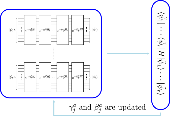
A general parallelized implementation of QAOA, or pQAOA, whose slices are obtained by considering r slice Hamiltonian Ha. In the figure, (leftvert {psi }_{a}rightrangle) are the initial states of each slice. We can note that no 2-qubits gates connect the slices that can, therefore, be executed parallelly. The pQAOA can be executed on (mathop{max }limits_{a}{n}_{a}) qubits, where na is the number of qubits involved in the slice Hamiltonian Ha. The slice samples (leftvert {tilde{psi }}_{i}rightrangle) are collected by measuring the slices and the global Hamiltonian H is evaluated according to eq. (6). Eventually, the parameters are optimized and the algorithm can proceed with the next iteration. In the figure, we use ({beta }_{j}^{a}) and ({gamma }_{j}^{a}), to show that since the slices are separated we can use different hyperparameters per slice. However, we can substitute each ({beta }_{j}^{a}) (({gamma }_{j}^{a})) with a unique βj (γj) to reduce the number of parameters to optimize.
After implementing the pQAOA, we collect the slice samples. Then, the hyperparameters are optimized by evaluating the global Hamiltonian as described in eq. (11). Notice that since σz and x are equivalent equation eq. (11) holds for the binary variables as well. Considering the slice samples as ({{{s}_{1}^{m},ldots ,{s}_{r}^{m}}}_{m = 1,ldots ,M}), where M is the number of slice samples collected, the evaluation of the global Hamiltonian can be done as for QAOA. Thus, if (leftvert tilde{psi }rightrangle) is the wavefunction obtained by executing QAOA, the evaluation of the global Hamiltonian is an approximation of the expectation value of H over (leftvert tilde{psi }rightrangle), that is
Notice that since we minimize the global Hamiltonians, we do not necessarily seek the global minima of the slice Hamiltonians. Therefore, all the theoretical guarantees of QAOA are lost. However, we can note that using the parallel implementation is reducing both the number of 2-qubits gate and the depth of the circuits. The number of entangling gates in the QAOA ansatz scales as ({mathcal{O}}(p{N}^{2})), where N is the number of qubits in the circuit and p is the number of layers applied. For pQAOA the number of 2-qubits gate scales as the number of qubits in the slices. Thus, if n is the number of qubits needed to implement the slices and r is the number of slices, then the number of entangling gates scales as ({mathcal{O}}(rp{n}^{2})). Moreover, the depth of the circuit depends only on the number of qubits and layers involved. Thus, since the slices are classically separable the depth scales as ({mathcal{O}}(p{n}^{2})) for pQAOA, whereas it is ({mathcal{O}}(p{N}^{2})) for QAOA.
A parallelization for quantum annealing (pQA)
Quantum annealing (QA) is one of the original quantum optimization algorithms designed to solve combinatorial optimization problems by exploiting adiabatic evolution, both in simulation and in programmable quantum hardware, known as quantum annealers34,35. The algorithm operates as follows: a quantum system (or a simulation) is initialized to an easy-to-prepare ground state (of the initial Hamiltonian Hi) and is then evolved to represent a different Hamiltonian (final Hamiltonian Hf) to be minimized. The result is a metaheuristic optimization algorithm that can be used to simulate quantum Hamiltonians. In-depth technical works on the physics behind quantum annealing theory and its implementation in hardware can be found in:36. For the purposes of implementing a parallelized version of QA, we only introduce the necessary components for constructing our algorithm, and encourage the interested reader to review the works cited above for more information.
The most commonly used Hamiltonian for quantum annealing is known as the transverse-field Ising Hamiltonian:
Here, s = t/τ ∈ [0, 1] is referred to as “normalized time”, and τ is the duration of evolution, an input parameter to the algorithm. The initial Hamiltonian shown here is ({H}_{i}={sum }_{i}{sigma }_{i}^{x}) and the final Hamiltonian Hf is the Ising Hamiltonian with spin variables ({sigma }_{i}^{z}), as described in eq. (9). The objective of the QA algorithm is to minimize Hf. A review of previous work in applying quantum annealing in practice can be found here7.
In current quantum annealing hardware, not all the connections between the qubits of the quantum system can be realized. We describe the connectivity of the qubits in the quantum annealer with a graph, where nodes represent the qubits and edges the connections between the qubits— we call this graph the hardware graph, or topology. Thus, not all the Ising Hamiltonian written as in eq. (9) with arbitrary connectivity can be directly implemented in the quantum annealer, since, in general, the geometry of the problem Hamiltonian graph does not match the topology of the quantum hardware. Therefore, the Hamiltonian must be reformulated to an equivalent Hamiltonian whose graph is compatible with the hardware graph. The problem of finding such an equivalent Ising Hamiltonian is called the minor embedding problem. The core idea is to identify every node of the problem Hamiltonian graph with a sub-graph of the hardware graph— these sub-graphs are called “chains of qubits”. Since the two formulations must be equivalent, two chains representing two neighbors of the problem Hamiltonian graph must be connected by at least one edge. This problem is known to be NP-hard and different heuristics have been developed to solve it37. Nevertheless, finding such an equivalent formulation is time-consuming, and since the most-used heuristics are not deterministic, being able to implement large-sized problems is challenging.
We now focus on motivating one method of constructing a parallel implementation of a variational version of QA by exploiting a parameter known as “annealing offset”. This specific parameter allows for the advancement or delay of the point in (normalized) time at which each qubit in the quantum annealer starts its evolution from Hi to Hf. This shift is denoted by Δi for qubit i, with Δi > 0 being a delay, and Δi < 0 being an advancement. Due to the changing eigenspectrum generated by the evolving Hamiltonian, it is known that some qubits in the system experience a slowdown in tunneling dynamics before the termination of the evolution, an effect known as “freeze-out”. This is known to affect the performance of QA as it makes it harder for the system to remain in the ground state38,39. The annealing offset parameter can therefore be used to change the freeze-out point on a per-qubit basis, in an attempt to mitigate this effect by synchronizing the freeze-out points. It has been demonstrated in quantum annealing hardware that tuning these parameters can (sometimes significantly) improve the probability of observing the ground state of Hf40,41,42. In general, however, given that the offsets are continuous parameters with non-convex search space, tuning these parameters optimally is a hard problem in itself.
We can implement a parallelized version of QA (pQA) using the framework presented above. We start by constructing the global and slice Hamiltonians for our optimization problem. Since QA is a continuous evolution of a quantum system, it is an analog device specifically designed to minimize a given Ising Hamiltonian. Therefore, we can consider the slices as subsystems of the quantum annealing system. Specifically, we identify the slices as the minor-embedded Hamiltonians of the slice Hamiltonians. For each slice, we assign a hyperparameter ({theta }_{j}^{a}), where a is the slice index and j is the chain index within the slice, to parameterize the annealing offsets for each chain of qubits in the minor-embedded problem. We can set the annealing offset for each spin in a slice a and chain j by setting it as ({Delta }_{j}^{a}={{boldsymbol{alpha }}}_{j}^{a}left(1-{theta }_{j}^{a}right)+{{boldsymbol{beta }}}_{j}^{a}{theta }_{j}^{a}), where ({{boldsymbol{alpha }}}_{j}^{a}=max {underset{{j}_{0}}{overset{a}{alpha }},ldots ,{alpha }_{{j}_{n}}^{a}}), ({{boldsymbol{beta }}}_{j}^{a}=min {underset{{j}_{0}}{overset{a}{beta }},ldots ,{beta }_{{j}_{n}}^{a}}) and where ([{alpha }_{{j}_{i}}^{a},{beta }_{{j}_{i}}^{a}]) is the annealing offset range of the i-th spin in the j-th chain of slice a. Then, we tune them independently within each slice using the global Hamiltonian as the target function, computing it as in eq. (6). A graphical representation of this process is shown in Fig. 3. For the tuning and search process of optimal offset parameters, we may use a procedure similar to the one in42 which uses a stochastic evolutionary algorithm to find improved annealing offset values with a limited budget (samples from the quantum annealer) or any other black-box optimizer. In Fig. 3, a general graphical description of pQA is shown.
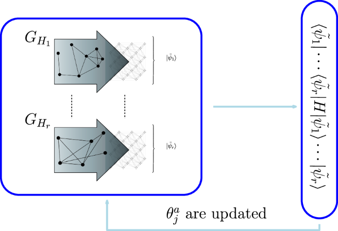
The parallel implementation of a variational version of QA, or pQA, whose hyperparameters (({theta }_{j}^{a})) are used to compute the annealing offsets. For each slice Hamiltonian, represented as a graph (({G}_{{H}_{a}})) in the picture, we compute the equivalent Hamiltonian compatible with the topology using minor embedding. Then, each chain of qubits is associated with a hyperparameter used to compute the annealing offsets of the qubits in the chain. We execute QA for each slice, represented as a minor-embedded problem, by evaluating it with the annealing offsets obtained with ({theta }_{j}^{a}). Then, the system is measured, the slice samples (leftvert {tilde{psi }}_{a}rightrangle) are collected, and the global Hamiltonian H is evaluated. Eventually, the annealing offsets are updated according to the new found ({theta }_{j}^{a}).
The parallel implementation has a significant physical effect on the annealing offsets optimization. Since each slice is embedded on the quantum annealer independently, we only attempt to mitigate the freeze-out within each slice. Furthermore, because we are not necessarily interested in the global optimum of each slice, and instead allow the independent slices to settle in local optima, we may not need to mitigate the freeze-out effect entirely, thus optimal offsets may be easier to find.
A parallel implementation of the variational quantum eigensolver (pVQE)
The variational quantum eigensolver (VQE) is a hybrid quantum-classical quantum algorithm that solves the minimum eigenvalue problem. For a given initial state and choice of parameterized ansatz, a quantum circuit is defined to iteratively adapt the ansatz parameters to minimize a target objective function. Specifically, given a unitary representation of the ansatz, U(α), where ({boldsymbol{alpha }}=left({alpha }_{1},ldots ,{alpha }_{q}right)), VQE attempts to solve:
where (leftvert psi ({boldsymbol{alpha }})rightrangle =U({boldsymbol{alpha }})leftvert 0rightrangle) is the ansatz applied to the initial state (in this case the zero state (leftvert 0rightrangle)), and H is a Hamiltonian whose minimum eigenvalue we wish to find (or approximate). In Fig. 4 we sketch the layout of a general VQE quantum circuit. Originally proposed in43, VQEs have been used in practice to solve a variety of problems in quantum chemistry and combinatorial optimization43,44,45. However, similar to other VQAs, VQE suffers from the same limitations of qubit count, circuit depth, and parameter optimization which limit its usefulness in applications. To overcome this, using our parallelization framework, we propose a variant, pVQE, which we outline here.
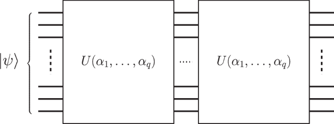
A graphical representation of a VQE circuit. We initialize the circuit with an initial state (leftvert psi rightrangle) and, then, we apply L times the unitary gate representing the ansatz of the VQE U(α1, …, αq).
One of the strengths of VQE is the freedom in the choice of ansatz. The goal is to construct an ansatz that can simultaneously be expressive enough to explore the Hilbert space of the circuit as well as be easily implementable46. Henceforth, we consider the hardware-efficient ansatz (HEA), a common choice of ansatz for VQE due to its ease of implementation47. For L layers of the VQE circuit with N qubits, we have ({mathcal{O}}(NL)) parameters and ({mathcal{O}}((N-1)L)) entangling gates. We stress that the ansatz of VQE HEA depends only on the number of qubits and it is, therefore, problem-independent. Thus, in this case, we can implement slices that have as many qubits as the number of spin variables involved in each slice Hamiltonian. This results in r classical separable circuits, where r is the number of slice Hamiltonians, with L repetition of the HEA with different hyperparameters. Then, as for the previous algorithms, the circuits are measured, the global Hamiltonian is evaluated, and the hyperparameters are updated by using a classical optimizer. The pVQE is shown in Fig. 5.
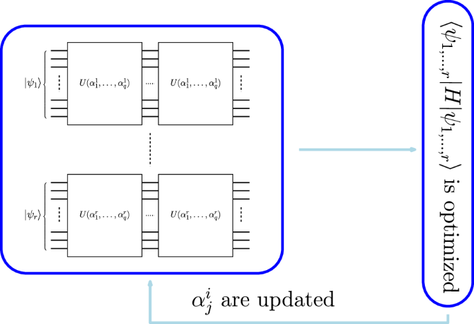
A parallelized implementation of a VQE, or pVQE. Each slice is initialized with the state (leftvert {psi }_{a}rightrangle). We apply L times to each initial state the unitary gate of the VQE (U(αa)) initialized with different sets of hyperparameters ({{boldsymbol{alpha }}}^{a}=({alpha }_{1}^{a},ldots ,{alpha }_{q}^{a})). The circuits are, then, measured, the slice samples (leftvert {tilde{psi }}_{i}rightrangle) are collected, and the hyperparameters are optimized by evaluating the global Hamiltonian H.
The main advantages are a reduction in the number of entangling gates and a decrease in the circuit depth. Suppose we have r slices that involve the same number of qubits (n). In that case, we can see that we need only n qubits to be able to implement the algorithm, the number of gates scales as ({mathcal{O}}(r(n-1)L)), and the depth of the circuit now only scales as ({mathcal{O}}((n-1)L)), since not all the qubits are connected anymore.
Performance from noiseless simulation
In Fig. 6 we show the performance comparison between different implementations of QAOA based on the method we described in section 2.2.1 obtained with noiseless simulation on GPUs and a classical benchmark. This algorithms are evaluated by solving 50 instances of the VRP problem with 3 locations and 2 vehicles. For every implementation, we consider only the best solution obtained for each instance. We solve the problem with: QAOA; multi-angle pQAOA; pQAOA, as described in section 4, where every slice has the same hyperparameters; single-slice pQAOA; and, the VRP tailored heuristic developed by Google OR. The global samples are retrieved using the selective rule to evaluate the result. The descriptions of the different implementations of QAOA can be found in section 4.
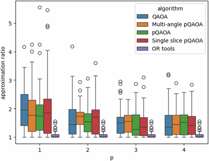
This figure presents the approximation ratio of 50 instances of the VRP with 2 vehicles and 3 locations. The boxes represent the upper quartile (top line), median (central line) and lower quartile (bottom line), and the whiskers extend to 1.5 times the interquartile range. The circles stand for the outliers. After training the hyperparameters, we collect the slice samples from the slice implemented with the best hyperparameters found. We select the best solution for each instance of the VRP and compute the approximation ratio using the optimal energy found with a brute-force method. The performances of the pQAOA are compared both with QAOA and a classical heuristic solver. We can see that the pQAOAs obtain the best solutions among the quantum algorithms in most cases. Albeit the improvement over the previous algorithm, the classical heuristic still performs better for this set of instances. In addition, we note that the pQAOAs obtain better quality solutions by increasing p, as QAOA.
To create the parallel version of the QAOA ansatz used to solve the VRPs, we apply the slicing as shown in eq. (14). Every implementation of QAOA is trained by collecting 10p+2 samples per circuit and by using 100p iteration to optimize the hyperparameters, where p is the number of layers. In our simulation, the number of samples used to train the hyperparameters and the maximum number of iterations are chosen such that the resources are adequate to produce better results for QAOA when p is larger.
The results presented in Fig. 6 show that the pQAOAs can achieve, especially for small p, better quality solutions than QAOA. Furthermore, we can see that the quality of the solutions obtained with pQAOA increases by increasing p as for QAOA. Thus, by employing our framework to parallelize QAOA we can approximate and most of the time overcome the performance of QAOA using the same resources to train the hyperparameters. However, it is worth mentioning that the classical heuristic beats every implementation of QAOA. Thus, either the number of samples used to train is not enough and, therefore, the optimum set of parameters is not reached or p is too low and therefore such quality of solution cannot be reached.
Moreover, to study how much information is lost due to the slicing of the problem we can look at the performance of QAOA when it is executed by using hyperparameters trained with one of its parallel implementations. In Fig. 7, we can see how the performance of QAOA changes with the different executions with different p and hyperparameters trained with different implementations. Notice that whereas the performances of QAOA are similar for p = 1, the quality of the solutions of the different implementations start differing when p is larger. Therefore, we can see that when p = 1 we can approximate the behavior of QAOA using the same resources, but the same cannot be said for larger p. This phenomenon can be attributed to the lack of approximation of the slices. The more layers we add to the slices, the more they differ from the original ansatz.
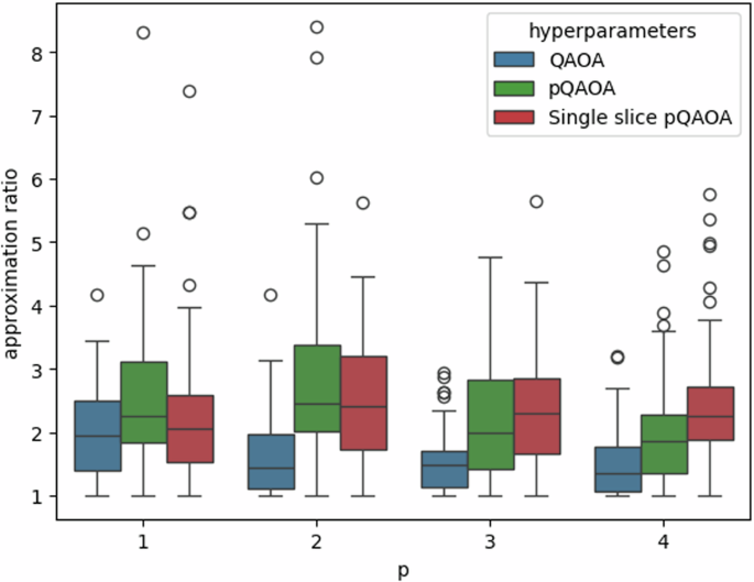
This figure presents the approximation ratio of 50 instances of the VRP with 2 vehicles and 3 locations. The boxes represent the upper quartile (top line), median (central line) and lower quartile (bottom line), and the whiskers extend to 1.5 times the interquartile range. The circles stand for the outliers. We compare the results of QAOA from Fig. 6 with the result of QAOA circuits evaluated with hyperparameters trained with different parallel implementations of the QAOA circuit. We can see that for small p the quality of the solutions obtained is similar. Thus, we can approximate the optimization of the hyperparameters of QAOA without implementing the whole circuit, but only using a parallel implementation. For larger p, the results start differing. This behavior can be linked to the difference between the quantum circuits. The more layers are implemented the more 2-qubits gates are removed from the QAOA ansatz. This changes the ansatz and can lead to different hyperparameters. However, it is worth mentioning that, even though evaluating QAOA with hyperparameters trained with pQAOA does not enhance the performance, it does not necessarily mean that the pQAOA cannot achieve better quality solutions.
Moreover, further analysis of the relationship between QAOA and its parallelized implementations can be found in the Supplementary Material. We present the relationship between the entanglement entropy between the subsystems involved in the slices for QAOA and pQAOA and the relation between the number of slices and the algorithm performances. Since these analyses are related to a small class of problems, no general conclusions can be drawn and broader analyses, that are out of the scope of this work, are necessary to identify general behaviors of the presented parallelized framework.
Experimental results
We present the results of the experimental implementation of the parallel framework presented, by solving 10 instances of VRPs with 10 locations and 3 vehicles on a quantum computer, IBM Brisbane Eagle chip48, and on a quantum annealer, D-Wave Advantage System 5.449. Since, as already mentioned, the slice Hamiltonians of the VRP are identical and due to the restricted access time provided, the experiments present an implementation of the single-slice pQAOA and the single-slice pQA. The global samples are retrieved using the vectorial rule to increase the number of solutions to evaluate. The single-slice pQA is realized as for the single-slice pQAOA, but the slices are obtained by finding the minor-embedded equivalent Hamiltonian of the unique slice Hamiltonian. We compare the best solution found by both algorithms with the classical solution obtained with Google OR tools, by considering the relative distance from it.
The training of the hyperparameters is conducted in two different ways. Due to the large queue time required to access the IBM quantum hardware to date, the hyperparameter could not be optimized directly on the hardware and, given the large number of qubits required to implement the parameterized quantum circuit (110 qubits to implement the unique slice), we could not simulate it classically. Therefore, to train the parameters of pQAOA we trained the single-slice pQAOA solving a VRP instance with 5 locations and 3 vehicles on a noisy simulation of the IBM Brisbane hardware. Due to the hyperparameter concentration effect50, we can consider the obtained hyperparameters to be close enough to the optimal ones. After training the hyperparameter, we implement the unique slice with p = 1 and p = 2 on the quantum hardware and collect 100 slice samples. The global samples are, then retrieved by using the vectorial rule. Since the gates used in our simulation are not native to the IBM quantum hardware, we used a heuristic provided by IBM that modifies the unique slice to make it implementable51. In Fig. 8, we show the results of single-slice pQAOA on real hardware. Conversely, regarding single-slice pQA, we train the hyperparameter with the quantum annealer using 600 iterations and collecting 100 slice samples for each iteration. The results of single-slice pQA are shown in Fig. 3.
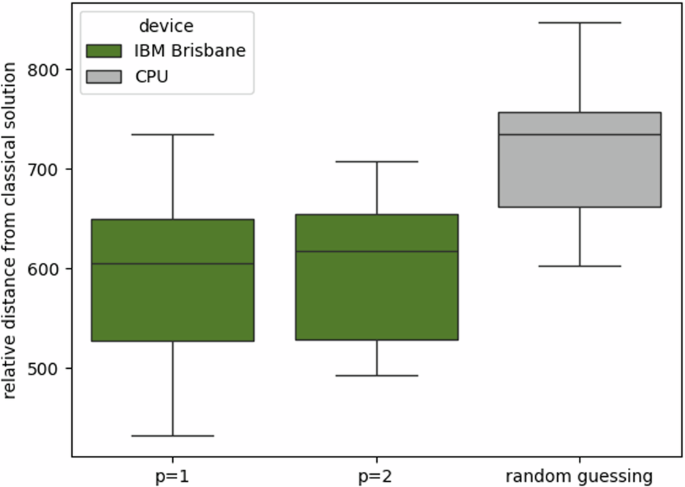
Relative distance from the classical heuristic solution of the best solutions found by executing single-slice pQAOA for the IBM Brisbane chip on 10 instances of VRP with 10 locations and 3 vehicles. The boxes represent the upper quartile (top line), median (central line) and lower quartile (bottom line), and the whiskers extend to 1.5 times the interquartile range. We execute single-slice pQAOA with p = 1 and p = 2. The boxes represent the upper quartile (top line), median (central line) and lower quartile (bottom line), and the whiskers extend to 1.5 times the interquartile range. The circles stand for the outliers. Due to restricted time access to the machine, the hyperparameters of pQAOA could not be trained directly by using the quantum hardware, instead, they were trained classically on a smaller instance on a simulated version of the Brisbane device. Thus, the results might be affect both by the non-optimal parameters and by the noise of the hardware. Furthermore, the results are compare to the best solutions found with random guessing, and it can be seen that, even though the results are worsen by the noise, they overcome the random guessing.
We note that the instances considered are large enough to make the direct implementation of the VQAs hard. For the implementation into the quantum annealer, the large number of qubits required and the high connectivity of the problems make finding a solution to the minor embedding problem for the global Hamiltonian hard. We stress that this problem is likely to be impossible to solve by using a direct implementation of QA. The number of qubits needed to implement the equivalent Hamiltonian with current minor embedding techniques scales as ({mathcal{O}}({n}^{2})), where n is the number of spins of the Hamiltonian to embed. Thus, to embed the VRP problem with 330 spin variables we need in the worst-case scenario 108.900 qubits, that are not available in current quantum annealers. Thus, we are not able to solve the instances considered with QA. On the other hand, for the IBM quantum hardware, the number of qubits required to implement QAOA is larger than the number of qubits available. Thus, a direct implementation of QAOA is not possible.
The results presented in Fig. 9 show several executions of pQA. To test that the parallelized framework works and can lead to improvement in the solution quality, we execute pQA with different settings. We implement pQA with two different annealing times 0.5μs, the fastest annealing time implementable, and 20μs, the standard annealing time set on the D-Wave quantum annealer. Furthermore, to stress that the optimization of the annealing offsets does improve the results, we first execute single-slice pQA by setting all the annealing offsets to 0, which is the standard setting for the quantum annealer, and, then, we compare the results with the trained hyperparameters. We can see that the results with the trained parameters reach better performance and that the best results are given with the trained parameters with annealing time 0.5μs. Moreover, pQA with optimized annealing offsets and annealing time 20μs does not show significant improvement compared to the execution without optimization. We think this is due to the thermal effects. When the annealing time is long enough, the thermal bath couples with the system and classical thermal effects take a major role in the computation. Thus, the freeze-out effect on the spins does not notably influence the performance of QA. Therefore, optimizing the annealing offsets in the presence of strong thermal effects reduces the improvement of the results. Furthermore, in this case, the classical heuristic reaches better results for each instance and the results are at least 10 times better than the best solutions found with pQA.
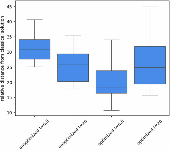
Relative distance from the classical heuristic solution of the best solutions found by executing single-slice pQA on the D-Wave Advantage 5.4 quantum annealer for 10 instances of VRP with 10 locations and 3 vehicles. The boxes represent the upper quartile (top line), median (central line) and lower quartile (bottom line), and the whiskers extend to 1.5 times the interquartile range. We execute single-slice pQA, by using an annealing time of 0.5μs, which is the fastest annealing process implementable, and 20μs, which is the standard time for the quantum annealer. The algorithm was trained directly on the quantum annealer by collecting 100 slice samples for iterations. The maximum number of iterations used was 600. Then, the performance is compared with a version of single-slice pQA, where the annealing offsets of every qubit involved in QA are set to 0. We can note that training the annealing offset of the slices brings to an improvement of the solutions, especially when the annealing time is 0.5μs. Despite the improvement, we can see that the performance is still worse than the classical heuristic solutions.
Conversely, the performance of the pQAOA executed on IBM quantum hardware is close to random guessed solutions. In this case, even though the optimization of the parameters is not done by using samples collected from the hardware, the bottleneck is the noise. Since the problems are densely connected, the depth of the circuit scales with the square of the number of qubits, ({mathcal{O}}({N}^{2})), thus, in this case, the depth of the algorithm results in the order of thousands of gates. Therefore, even though the problem is reduced by applying the slicing, the algorithm fails to mitigate the noise of the quantum hardware. Thus, since the number of used gates exceeded the error tolerance of the device, error mitigation techniques could have been used to reduce the noise effect. Due to the framework’s flexibility, error mitigation can be applied either during the creation of the slices or to an already error-mitigated algorithm. Thus, after computing the slice Hamiltonians, we could have implemented QAOA circuits enhanced with error mitigation52; or, the error mitigation algorithm can be considered the original VQA and sliced according to the presented parallel framework.
Error mitigation techniques were not tested in this work due to limited access to the machine.
Moreover, it is worth noticing that the slicing is not done optimally but it is inferred by the inspection of the problem itself. Therefore, new ways of slicing with smaller slices can lead to improved solutions.
Furthermore, the results of the two different quantum hardware are hard to compare since the IBM machine is a universal quantum computer, whereas the D-Wave quantum annealer is designed specifically to find the minimum energy state of Ising Hamiltonians.
Nevertheless, due to restricted access time, no further experiments were possible. However, the pQA results suggest that the application of our framework can lead to improvement and shrink the gap between the performance of quantum hardware and classical algorithms. Furthermore, different slicing should be tried and larger problem instances, especially implemented into D-Wave annealers, should be investigated. Conversely, for IBM quantum hardware, more efficient VQA to solve optimization problems should be tested, to verify whether a smaller number of gates makes the mitigation of noise possible.
Discussion
In this work, we presented a framework to create parallelized versions of variational quantum algorithms. Especially, we show how to implement parallelized versions of variational quantum optimization algorithms informed by the optimization problem directly. Our analyses were focused on QAOA and a variational version of QA, but they can hold for all VQAs solving optimization problems encoded as Ising Hamiltonians. The presented framework allows the implementation of quantum algorithms that require more qubits than are available. Therefore, we can maximally exploit the reduced number of qubits in small quantum processors and scale the algorithm to tackle larger problems. Specifically, we show how to solve constrained optimization problems by exploiting their geometrical properties to identify the slices for pQAOA and pQA. Furthermore, we noted that the slicing method yields an exponential set of global samples. While this can be advantageous when access to the quantum hardware is limited, we proposed a rule to select the global samples to reduce the complexity cost of our parallelized algorithms in the case that collecting the samples from the quantum hardware does not represent an issue.
We solved 50 different instances of VRP with 3 locations and 2 vehicles with different implementations of pQAOA, showing that not only our parallelization framework can approximate the QAOA, but that, for some implementations, we can even reach better performance. We found that especially for low-depth circuits (specifically for p = 1, 2) pQAOA is better than QAOA. Conversely, for larger p the performance of pQAOA becomes similar to QAOA. Furthermore, we evaluated the QAOA circuit with hyperparameters trained by pQAOA to understand how well the parallelized version can approximate QAOA behavior. We conclude that, while for p = 1, the performance of the QAOA circuit evaluating different trained hyperparameters coincides, with the repetition of the layers the circuits begin to differ significantly and, thus, pQAOAs cannot approximate the original QAOA well enough. On the other hand, as already observed, we stress that this does not necessarily mean that the parallelized algorithms perform worse than the QAOA.
Moreover, we tested our framework on real quantum hardware by implementing single-slice pQAOA on the IBM Brisbane chip and single-slice pQA on the D-Wave Advantage system 5.4 quantum annealer. We analyzed the algorithm performance based on 10 instances of VRP with 10 locations and 3 vehicles against the solutions obtained with a classical heuristic solver. By employing our framework we obtained different advantages: for the IBM quantum hardware, we solved a problem that could not be solved by using other implementations of QAOA since it requires more qubits than are in the quantum hardware; and, for the D-Wave quantum annealer, we solved a problem that would be hard to implement directly into the quantum annealer, because its minor-embedded version is hard to find. In addition, we observed that we could improve the solution obtained with the quantum annealer. Conversely, the noise of the IBM quantum computer affected the results showing that the depth of the implemented circuits was too large and caused noise effects to play a major role in the computation.
We conclude by stressing that our parallel implementation shows improved results compared to the non-parallelized version of the algorithms. Even though the results are not competitive against the classical heuristic, we expect different behavior for larger instances that are hard to solve with the classical heuristic.
In future works, we will investigate possible applications of the parallelization framework beyond solving optimization problems. Moreover, since the slicing results in a modification of the ansatz, we will address the consequences of this modification by investigating the effect of barren plateaus, and the relationship between performance and lost entanglement entropy influenced by the choice of the slicing.
Methods
Slicing combinatorial optimization problems: the vehicle routing problem
We now present how to apply slicing to VQAs that solve combinatorial optimization problems formulated as Ising Hamiltonians. To identify tailored slices of the VQA quantum circuit, we have to exploit the properties of the Ising Hamiltonian formulation. We can write an arbitrary Ising Hamiltonian as:
where ({h}_{i},{J}_{ij}in {mathbb{R}}) with Jij = Jji and ({sigma }_{z}^{i}) are spin variables that can take values of either + 1 or − 1. Notice that, since the terms that appear in H are at most of quadratic order, we can represent the Ising Hamiltonian as a graph where nodes represent the spin variables ({sigma }_{z}^{i}) and edges represent the quadratic terms ({sigma }_{z}^{i}{sigma }_{z}^{j}). Given this dual model description, we can use algebraic and geometrical properties to create problem-tailored slices. In this work, we focus on constrained optimization problems since most industrial-relevant problems belong to this class, and since their encoding as Ising Hamiltonian usually includes redundancies that can be used to identify the slices.
The following Hamiltonian can represent constrained combinatorial optimization problems:
where Hobj represents the objective function and HC is the Hamiltonian that encodes the constraints that define the feasible region of the problem. Both Hobj and HC are Ising Hamiltonian of the form as in eq. (9).
Let ({H}_{tilde{C}}) be the Ising Hamiltonian that implements part of the problem constraints. If, by removing ({H}_{tilde{C}}), the resulting graph representation of (H-{H}_{tilde{C}}) is disconnected, we can consider each connected component as a distinct Ising Hamiltonian. Therefore, we can use these Hamiltonians to create the slices of the VQA quantum circuit. To differentiate, we call the original Hamiltonian representing the combinatorial optimization problem the “global” Hamiltonian, whereas we call the disconnected Hamiltonians, the “slice” Hamiltonians. Therefore, according to the VQA, we can implement different circuits based on the slice Hamiltonians. We can see that the circuits created in this way are separable and, therefore, eq. (1) is satisfied. We can apply the same argument as in29 and recover the lost information in the slicing using the global Hamiltonian as the objective to update the hyperparameters. Since the slices do not contain information about ({H}_{tilde{C}}), the classical optimizer must evaluate the global Hamiltonian H so that the minimal solutions obtained belong to the feasible region defined by the constraints encoded as ({H}_{tilde{C}}). Therefore, even though the slices represent only part of the original problem, the classical optimizer is driven by the global Hamiltonian towards its minima. In addition, we can note that we can consider the spin variables ({sigma }_{z}^{i}) as independent random variables, and therefore when we evaluate the global sample (leftvert {s}_{1},ldots ,{s}_{r}rightrangle), as defined in eq. (2), we obtain
Thus, the exponential overhead of global samples does not represent an issue for the parameters training, because we can compute the expectation value of ({sigma }_{z}^{i}) over the slice samples collected from the slice implementing the slice Hamiltonian where ({sigma }_{z}^{i}) belongs to.
We now examine the Vehicle Routing Problem (VRP), a well-known NP-hard optimization problem, to show how to apply the slicing process described above. In the VRP, we consider a fleet of vehicles that delivers goods or services to customers. The goal is to find the optimal set of routes that minimizes the costs associated with the deliveries. We can describe the problem as a weighted graph in which the nodes represent the locations to be visited and the edges represent the possible connections between the locations. The objective becomes to find the path for each vehicle so that each location is visited exactly once by a vehicle and the sum of the costs associated with the edges is minimized. In this variant, the vehicles start and end from an initial location, called “depot”. We can write the QUBO formulation of the VRP as follows53,54,55:
with
where the locations to visit, i, are numbered from 0 to n and 0 is the depot; wi,j are the costs associated with reaching location j from location i and (W:= mathop{max }limits_{i,j}{w}_{i,j}); A is the number of vehicles in the fleet; and, the index s represents the discrete step of the process. It is worth noticing that, in this case, the variables xa,i,s are binary variables that can take values of either 0 or 1. As mentioned above, the QUBO formulation of a problem is equivalent to its Ising Hamiltonian model. To write eq. (12) as eq. (9), we have to apply the substitution ({x}_{a,i,s}=2(1-{sigma }_{z}^{a,i,s})). Nevertheless, since both formulations involve at most quadratic terms, their graph representations are isomorphic. Thus, we can use both formulations interchangeably.
We now show how to find the slice Hamiltonians starting from the VRP QUBO. In eq. (12), we can see that only the addend
contains quadratic terms that involve different indices for the vehicle, a. Thus, if we remove those terms, the graph representation of the problem has no edges that connect two nodes representing the variables xa,i,s with different a. Therefore, the components of the graph are disconnected and represent the slice Hamiltonians.
We can see how to identify these components by considering the algebraic description of H. We stress again that only eq. (13) involves different a in the quadratic terms. Therefore, we can write:
and by considering
we can summarize H as:
Therefore, Ha are the slice Hamiltonians of the problem and Hc is the Hamiltonian ({H}_{tilde{C}}) that is only considered by the classical optimizer.
In the following section, we describe how to create the slices based on the decomposition of the Hamiltonian applied to different VQAs presented above. Nevertheless, different properties of the problem could be used to obtain the slice Hamiltonians. In the Supplementary Material, we present how to find the slice Hamiltonians of the global Hamiltonian that encodes the MaxCut problem by exploiting the k-connectivity of the graph.
Implementation description
We use different parallel implementations of QAOA, as presented in section 2.2.1. Each implementation depends on the choice of the number of hyperparameters to train in the circuit. In the following subsections, we describe the implications of such a choice.
Multi-angle pQAOA
After identifying the slice Hamiltonians, each slice is implemented as a separate quantum circuit. The original QAOA circuit contains 2 parameters per layer, but now, since there are no 2-qubits gates connecting the slices, one can decide to assign independent parameters per slice. This yields 2rp hyperparameters to optimize, where r is the number of slices and p is the number of layers of the QAOA circuit.
Single-slice pQAOA
Instead of assigning different hyperparameters per slice as described above, one can keep the same number of hyperparameters as for the original QAOA. Notice that, when the slice Hamiltonians have the same graph representation, this yields a different implementation of pQAOA. If the slices are identical, and the same hyperparameters are used for every slice, then sampling from the different slices is equivalent to sampling more from one single slice. Therefore, we can implement one unique slice and retrieve the global Hamiltonian solutions by considering the Cartesian product of the samples with themselves. Thus, if the optimization is encoded on a Hamiltonian defined on N = rn qubits, where r is the number of identical slices, we can approximate such Hamiltonian using only n qubits. Therefore, we call this version of the algorithm, single-slice pQAOA.
In addition, we henceforth refer to a parallel implementation of QAOA implemented with 2 hyperparameters per layer, as for the original implementation of QAOA, as pQAOA.
As discussed in Section 2.1, collecting the global samples to evaluate the solutions must be done according to a rule. After collecting the slice samples ({{leftvert {s}_{i}^{a}rightrangle }}_{i = 1,ldots ,M}), where i = 0, …, r and M is the number of measurements, we have to choose some samples from the vectorial product
During this work, we use the following rules. We can consider all the global samples in the vectorial product defining our global samples set as
or, we can enumerate them from 1 to M and retrieve one global sample from the slice samples with the same index, obtaining the global sample set
As already mentioned, if we use the rule eq. (15) the cardinality of the global sample set scales exponentially in the number of slices, that is ({mathcal{O}}({M}^{r})), whereas if we use rule eq. (16) it scales linearly in the number of measurements, that is ({mathcal{O}}(M/r)). For the sake of simplicity, we call rule in eq. (15) “vectorial” and rule in eq. (16) “selective”.
We first test the framework we developed by solving 50 randomly generated instances of VRPs with 2 vehicles and 3 locations using different parallel implementations of QAOA. The locations of the studied instances are generated with a Gaussian distribution over a discrete grid of 100 × 100. The depot is placed at the center of the grid, with coordinates (0, 0). The distances between locations are computed with the L2 norm. We use NVIDIA’s cuQuantum56 to simulate the quantum circuits executed on GPUs. Because of the relatively small sizes of VRP instances, we can calculate the global optima with a brute-force approach. Therefore, we compute the approximation ratios related to the brute-force solution to evaluate the quality of the solutions obtained using each implementation. The results obtained by the quantum algorithms are then compared to the open-source software package OR-Tools by Google57.
Eventually, we exploit our framework to solve 10 instances of VRPs with 3 vehicles and 10 locations on the IBM Brisbane Eagle QPU48. The locations and the depot are obtained as in the previous setting. This experiment applies our framework when the number of qubits needed to implement the problem (330) is larger than the number of qubits available in the hardware (127). Furthermore, we compare these results with the performance of a parallel implementation of quantum annealing on the Advantage system 5.449 quantum annealer used to solve the same instances. The quality of the solutions obtained from the experiments is evaluated by considering the approximation ratio related to the solutions obtained by using the OR-Tools solver.

Responses