Parallel scaling of elite wealth in ancient Roman and modern cities with implications for understanding urban inequality

As global urbanization accelerates through the Anthropocene, the interplay between sustainable development and inequality will be paramount for shaping future urban environments and policy. The technosphere—technology and anthropogenic structures—now weighs an estimated 30 trillion tonnes, much of which is concentrated in urban centers¹. This massive number reflects the magnitude of urban impacts on the Earth system, an impact that will surely grow with projections indicating over 70% of the global population will reside in cities by the year 2050². This trajectory means that charting a sustainable course is increasingly urgent. Recent developments, including the United Nations’ (UN) latest Sustainable Development Goals report³ and Nature’s recent comprehensive special collection on urban sustainability⁴, have highlighted many challenges and perspectives surrounding urban growth and sustainability. Chief among these are the challenges posed by the intersection between urban development and inequality. The UN expects that by 2050 there will be 2 billion more people living in slums in and around the rapidly growing urban centers of the world³, and many sustainability scientists have identified crucial links between inequality and barriers to sustainable development^5,6,7. However, the long-term relationships between urban growth, wealth, power and inequality are poorly understood, making predictions and planning difficult. Combining the settlement scaling theory^8,9 (SST) with recently developed and growing archeological and historical databases has the potential to greatly improve this situation.

The SST is a powerful framework for explaining and exploring relationships between urban growth and different economic, infrastructural and structural parameters⁹. It explains and predicts attributes of urban centers as a function of fundamental principles of human social interaction that scale with population size^8,10. Scholars have, for instance, found that larger settlements are, on average, not only more productive (for example, higher wages and more innovations) but also more costly (for example, higher rents), than smaller ones¹⁰. These scaling relationships are nonlinear such that increases in population size can lead to explosive increases in some urban traits. Crucially, SST focuses on the complex, nonlinear dynamics of urban systems rather than their initial conditions, very similar to how the aphorism ‘the rich get richer’ highlights wealth compounding without saying anything about how the rich got rich initially. Consequently, the theory describes scaling process and invokes nonlinear dynamics such as feedback, rather than simple linear causation, where one urban trait directly causes the other¹¹. According to the theory, these complex patterns arise naturally in a law-like manner—similar to metabolic scaling in organisms—as a function of small-scale interactions among individuals in the context of high-density urban systems that contain fractal, space-filling transportation and resource distribution networks. This premise has been supported in scaling analyses performed on modern cities and ancient examples alike, including, for instance, Aztec cities in the Basin of Mexico and Imperial Roman cities^8,10. Thus, individual cities—regardless of culture, technology, economy or time period—are revealed by SST to be manifestations of a general process that is inherently nonlinear and stochastic, while still exhibiting variations that are deeply influenced by contextual factors^12,13. This ‘urban process’ generates wealth greater than would be expected if individual contributions to aggregate wealth increased linearly with population growth, which, in part, explains the success, proliferation and attraction of cities through time and space, despite the costs and potential downsides urban dwelling.

Wealth scaling is a positive feature of the urban process, particularly given rapid trends toward urban life in the twenty-first century. More wealth per capita reflects efficiency gains, that is, economies of scale with respect to infrastructure⁹, and this greater efficiency may help deal with the challenges of population growth and finite resources. Moreover, more wealth means more resources available for climate change adaptation. Nevertheless, there is also abundant evidence that urban wealth gains are not distributed evenly^{14,15,16,17,18}. For instance, in modern cities such as San Francisco, the technology boom has substantially increased local wealth and also exacerbated housing affordability issues, widening the divide between urban high earners and other residents¹⁹. These disparities can be observed in the physical layout, architecture and monumentality of modern urban centers²⁰. Such inequality could challenge sustainable development, which is why many authors have advocated including ‘equity’ as a pillar of sustainability alongside ‘environment’ and ‘economy’⁵. It is also why the UN emphasizes inequality in the 11th global Sustainable Development Goal, to ‘Make cities and human settlements inclusive, safe, resilient, and sustainable’³. The ubiquity of inequality in modern urban centers, along with easy to find examples of inequality in past cities, raises important questions: While urban dynamics seem to generate wealth by its very nature, do cities also necessarily concentrate that wealth in the hands of a few elites as they grow? If so, how universal is this tendency across time given the various other important factors such as economic system (for example, capitalism versus something else), culture, technology and so on? And importantly for present purposes, is there a material expression of this tendency that affects urban environments? Answering these questions will be crucial for understanding a pillar of the modern sustainability concept and, by extension, for charting a path toward a sustainable urban future.

With these important questions in mind, we conducted an intertemporal comparative scaling analysis involving ancient Roman and modern elite wealth in urban centers. Our focus on Roman society during the first two centuries common era (CE) was motivated by recent studies suggesting its urban inequality mirrored that of some of today’s largest cities. For instance, Pompeii’s Gini coefficient, a measure of inequality, is estimated at 0.5–0.6 (refs. ^21,22,23) for the years near its demise in 79 CE, aligning with recent estimates for major US cities such as New York and Miami, both of which have estimates of ~0.51 or higher²⁴. The data on ancient Roman urban monumentality that could be compared with modern data are also readily available online, whereas we are not aware of comparable datasets for other preindustrial societies—though some could be created for ancient societies in the Americas, for instance. Similar to other scaling studies, ours involved comparing urban traits to population sizes using regression techniques. The key parameter of interest was the scaling parameter—a regression coefficient—which indicated how the evidence for urban elite wealth varied with population size.

Our study involves several analyses. First, we examined scaling between population size and urban elite wealth in the early Roman Empire. The two available datasets were counts of monuments (frequently sponsored by the elite^25,26) and counts of epigraphic inscriptions (honorific dedications, usually to elites and their family members²⁷), accessible through online databases. To account for idiosyncrasies in these archeological and historical datasets, we used novel, advanced, Bayesian versions of standard scaling regression models that accounted for the count-based nature of the data, uncertainties in population estimates and potential regional differences among Roman provinces^8,12,28,29 (Methods). We ran multiple analyses involving different subsets of the Roman cities database to explore possible biases. A key set of analyses involved excluding Roman cities with zero counts for monuments/inscriptions, which allowed us to explore the effect of zero inflation due to preservation, recovery and research biases present in archeological and historical data. Next, we examined scaling between population size and urban elite wealth in modern cities, also using two datasets. One included counts of exceptionally tall buildings (exceeding 150 m), which we consider to be an expression of both modern urban monumentality and signals of elite wealth concentration/competition^30,31 (for example, Trump Tower in New York or the Burj Khalifa in Dubai). The other was counts of billionaires residing in major cities. Lastly, we ran supplementary analyses to explore model fit, compare the power-law model to a reasonable alternative and examine the effect of outliers on our scaling parameter estimates.

Then, we developed an agent-based model (ABM) to explore how population scaling could potentially be linked to wealth inequality in terms of individual interactions so that the explanation would be compatible with the SST. We based the ABM on the Boltzmann wealth model, which posits that money, similar to energy in a closed system, is conserved and will over time become exponentially distributed³². Agents, representing (in the present case) all individuals living in an abstract city, bounce around (similar to gas molecules) randomly exchanging virtual money, which counterintuitively leads to substantial inequality. This simple model of agents bouncing into each other at random in a circumscribed space is a direct parallel to the ‘amorphous settlement’ model of the SST, from which more complicated complex infrastructural models were developed⁹. Our model, enhanced with simple network effects, starts by placing agents in a network, allowing money exchanges only with connected agents, and introduces a preferential attachment parameter to mimic real-world social and economic networks³³. By varying this parameter, we analyzed the impact of connection disparities on inequality, measured by the Gini coefficient, which we chose because of its simplicity and widespread adoption for measuring inequality past and present³⁴.

We reasoned that comparing the scaling parameters for proxies of elite wealth across time and culture could reveal fundamental similarities that transcend temporal, cultural, economic and technological divides. The Imperial Roman period’s surge in monumentality, driven partly by euergetism (elite benefaction and power signaling in the form of funding monumental building projects and repairs) and the increase in epigraphy highlight the ancient elites’ strategies for wealth display and status legitimation^26,27,35,36. Similarly, modern elite wealth and power has been signaled by a kind of patronage involving ambitious skyscraper projects for many decades³⁷. By juxtaposing ancient Roman practices with the present-day concentration of wealth produced by a very different economic system, with different technology, we aimed to uncover potentially enduring patterns in the scaling relationship between population size and elite wealth. And, lastly, with the our network-Boltzmann ABM as an heuristic aid, we sought to explain any identified scaling effects by developing an SST-compatible hypothesis for future testing.

The results of the analyses consistently indicated the presence of a power-law relationship between urban elite wealth indicators and population size (Table 1). In each analysis (see Methods for details), we found a positive relationship between the relevant elite wealth indicator and population size estimates. The models all had average R² values of around 0.15–0.57 (Table 1 and Fig. 1), which reflects data uncertainties and the likely possibility that more than just population size affects these indicators of elite wealth. It also clearly indicates that monuments (modern or ancient), inscriptions and even counts of billionaires are only a proxy for elite urban wealth with variability left over to explain by other factors. Most of the scaling parameter estimates had overlapping 95% credible intervals (CIs) spanning ~0.2–0.5 with some notable outliers, and most means are clustered in the region ~0.3–0.5. Our results also indicate that there was little difference among Roman provinces in terms of scaling coefficient (see Markov Chain Monte Carlo (MCMC) trace plots in ref. ³⁸ with filenames containing ‘provinces’).

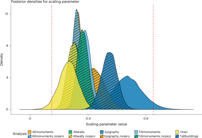
The vertical dashed lines represent theoretically predicted values from the SST discussed in the text. The left-most line corresponds to the scaling parameter expected of average individual wealth, while the right-most line indicates the value expected for infrastructure⁹.

Full size image

In addition, the supplementary analyses indicate that the power-law model should be preferred to the linear-log alternative (with 70–80% of cities being better predicted by the power-law model; ‘model_comparison.csv’ and ‘loo_est_…csv’ files in ref. ³⁸). We also found very few extreme outliers in the power-law model analyses—indicated by high Widely-Applicable-Information Criterion diagnostics (pWAIC) values reported by Nimble, Pareto Smoothed Importance Sampling Leave-One-Out Cross-Validation (PSIS-LOO), Pareto K values and residual-versus-predicted plots (‘resid_…png’ files in ref. ³⁸). Crucially, these outliers (extreme and moderate) had little impact on our parameter estimates (‘post_summary_…linlog.csv’ files in ref. ³⁸).

Lastly, our ABM results clearly showed that the strength of preferential attachment is positively correlated with inequality as measured by a Gini coefficient. By varying the preferential attachment parameter, we could see a clear correlation. Different degrees of preferential attachment led, as would be expected, to different degrees of connection bias. With low preferential attachment, a highly even network (uniform degree distribution) was obtained where most nodes/agents had roughly the same number of connections. In contrast, higher preferential attachment led to highly uneven (scale-free) connection distributions where connectivity was disproportionately concentrated in a few nodes. The latter corresponded to higher Gini coefficients indicating greater inequality (Fig. 2).

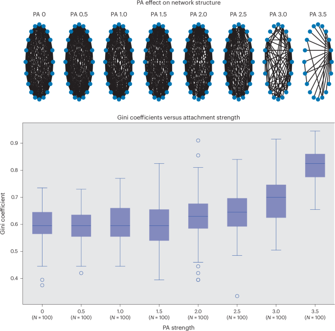
The boxes each refer to N = 100 Gini estimates for each level of preferential attachment (PA), which indicate the median and interquartile ranges (IQR). The whiskers indicate 1.5 times the IQR, and the circles are outliers beyond that range. As the plot indicates, increasing preferential attachment strength leads to increased Gini coefficients (greater inequality). The specific model settings chosen (the range of PA values explored and number of agents) were chosen so as to produce a clear image depicting the model dynamics. It should be noted that since Gini coefficients are bounded in [0,1], and PA values ultimately lead to a continuum between complete connectivity and a network where all agents are connected to only one super-connected agent, the expected relationship between the PA and Gini coefficient is actually S shaped, and increasing PA further reveals a smooth increase to an asymptote where the Gini coefficient is 1 (interested readers can explore these dynamics by running the Python code provided in the project repo in ref. ³⁸).

Full size image

Our results suggest that inequality may be a structural trait of the urban process that transcends time and sociocultural, technological and economic differences. We identified a pattern of increased wealth concentration that corresponds with increased urban population sizes across diverse indicators in societies separated by more than 1,000 years (Fig. 3). Moreover, the two case studies exhibit massive differences in culture, technology and economic organization. Yet, the values we estimated for the scaling coefficients in these two distinct cases are strikingly similar (Fig. 2). Thus, it seems reasonable to suspect that perhaps the same mechanisms that lead to superlinear wealth scaling in cities could give rise to wealth concentration, with all that entails for social and economic inequality.

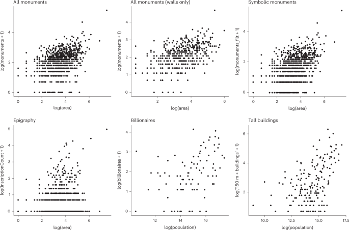
Note that we added a constant to the response (y axis) counts to create log–log plots consistent with previous scaling research.

Full size image

Our research, of course, has limitations. There are certain well-known challenges associated with identifying and proving the existence of scaling relationships in noisy real-world data^39,40. By scaling relationships, we generally mean that one variable is functionally related to another and a unit change in the first variable corresponds to a fixed unit change in the other regardless of the scale of the two quantities—that is, a relationship that holds at all scales and is, therefore, ‘scale invariant’. Such relationships are important because they imply universal functional relationships, which suggests a deep connection. In the context of SST, the existence of a power law implies that, say, the area of roads increases consistently in concert with population regardless of whether one considers a change from a small population to a large one or a change from a large population to an enormous one (though the relationship need not be linear). In real-world data—especially aggregated archeological and historical data—it can be difficult to distinguish between universal scaling and a relationship that holds only over some range of values or only in certain contexts³⁹. Importantly, with archeological and historical datasets, there is also a temporal palimpsest effect whereby data points corresponding to different times are aggregated, often to overcome sparse data problems or because of temporal uncertainties. For these reasons, our analysis, similar to many other scaling studies, cannot be taken as conclusive. Still, our first supplementary analysis (Methods) in which we compared the power-law models with a sensible alternative (linear log) indicated a clear preference for the power law. We also found, in our second supplementary analysis, no indication of outlier cities having affected our estimates of the scaling exponent. In addition, while the Oxford Roman Economies Project (OxREP) data spans from 100 before common era to 300 CE, most of the monuments and inscriptions date to the second century CE during a time of explosive urban growth throughout the Roman Empire^41,42. So, while we urge caution against overinterpreting our findings, they appear to be robust and indicative of scaling behavior.

Importantly, the consistency across data treatments was encouraging. The relationships we identified were consistent regardless of the way urban areas were estimated and even after filtering out features of debatable monumentality, such as street grids and fora/agorai and walls that could be confounding because of their use in our analyses to define settlement areas. The pattern was also consistent between the two different data types, monument counts and epigraphy and irrespective of differences in the way the relevant databases were compiled. A notable exception was the parameter estimate for the epigraphic database that included all of the zeros present in those data. The posterior distribution (Fig. 1) for the scaling parameter in that case is shifted upward compared with the bulk of the other estimates. This indicates that the presence of so many zeros still clearly had an effect despite our use of a statistical model often used to account for cases where count data contain potentially false zeros giving rise to ‘overdispersion’. The best explanation, we argue, is that the analysis in which we excluded zero counts of inscriptions is closer to the truth because we find it highly unlikely for any Roman settlement with city civic status—and, thus, in the database we used—to have had no epigraphy²⁷ (see Methods for further details). Crucially, for present purposes, the Roman scaling relationships were also remarkably close to, and had overlapping uncertainties with, the ones we identified in the data about modern elite wealth concentration and conspicuous, imposing monumentality in urban centers. So, while there is uncertainty about the specific scaling value, there appears to be some convergence across datasets, and importantly, none of the values seem to correspond with existing predictions from the SST. We take this convergence across data types and time periods as indicative of some as yet underexplored persistent process, making it an enticing empirical finding.

With the foregoing in mind, we can speculate about the particular scaling parameters we identified. Compared with most of the other empirical SST research and predictions made so far, the 0.3–0.5 range of parameter means we observed is unusual—see Hanson for a similar finding using a simpler model⁴³. Established SST predictions for socioeconomic productivity (outputs) focus on aggregate wealth (for example, total gross domestic product for a given city) and average wealth (for example, per-capita productivity), not the wealth of specific socioeconomic strata, as noted by other scholars¹⁷. For indicators of aggregate wealth, the theoretical scaling parameter would be (frac{7}{6}), and for per-capita wealth the parameter would be (frac{1}{6}). These values indicate superlinear and sublinear scaling of wealth, respectively, and reflect primarily the gains from increased total numbers of interactions and increased per-capita interaction rates in larger cities. They also arise as a result of cost savings from economies of scale making movement (and other aspects of urban life) more efficient for larger cities.

The value range we estimated from our case studies, however, is lower than would be expected of aggregate wealth and higher than expected of average per-capita wealth. Since monuments and dedication inscriptions were frequently funded by wealthy individuals for symbolic and political reasons in the Roman Empire^27,35, they do not reflect aggregate or per-capita wealth. Likewise, counts of billionaires in modern cities or extremely tall buildings do not reflect the typical wealth of urbanites in those places. Rather, these indicators reflect the wealth of only the wealthiest citizens, which could explain why we observe a scaling parameter different than any comparable wealth or infrastructure prediction from the SST for structured settlements⁹. The value range is notably higher than would be expected of the (frac{1}{6}) value representing average per-capita wealth scaling. Intuitively, a higher value makes sense given that individuals with more wealth tend to gain more from increased interaction opportunities and larger markets than individuals with less wealth. There is a limit to this, though, since the scaling parameter we estimated is sublinear, meaning that urban expressions of elite wealth concentration grow more slowly than population. This implies that there are ‘diminishing returns’, which aligns with previous research on ancient inequality showing that the magnitude of inequality may be smaller in the largest cities²². Nevertheless, these patterns reinforce the old adage that ‘the rich get richer’, an unfortunate dynamic that may have been as true in the past as it is today.

This scaling pattern, we think, may be driven by network effects acting on interaction rates in urban centers. The SST is based on the idea that interaction rates affect a variety of measurable urban traits (for example, economic transactions, innovations, patent filings, crime and disease outbreaks), and interactions in urban centers are catalyzed by increased population density (more people interacting in a given space) and efficiencies gained by space-filling infrastructure networks (allowing individuals to interact efficiently across the urban space). Since interactions provide benefits, increased average per-capita interaction rates are the source of the many superlinear scaling effects observed for socioeconomic outputs, such as wages and patents. However, the SST does not say anything explicitly about expected patterns in cases with differential access to the social networks.

Our ABM simulations indicate that our proposed explanation is plausible and could be used to extend the SST. The results showed that connection inequality exacerbated wealth concentration substantially (Fig. 2). These findings underscore the importance of considering not only the physical (complex, space-filling) infrastructure of urban centers but also the structured nature of human social networks, highlighting a potential pathway for extending the SST to more accurately reflect real-world dynamics. As explained earlier, the SST explains observable scaling between population and various urban traits (including wealth) as a function of lower-level population-interaction probability scaling, where there is no connection variability among individuals. Our network model shows what can happen to wealth distribution when the assumption about connection quality is relaxed or stressed. Based on these simple findings, we argue it is possible that the interplay of urban infrastructure networks and human social networks gives rise to unequal access to interaction in urban centers, thereby creating the observed scaling effects—though it should be noted that a number of potential processes beyond simple preferential attachment could produce connection inequality, and those should be explored in future SST research on inequality.

To our knowledge, our research revealed the first potential evidence of urban scaling in elite wealth and power displays that transcends millennia, economics, culture, political organization and technology^17,28. Using a robust Bayesian approach to account for historical uncertainties and spatial effects and combining archeological and historical data with modern data has opened up new avenues for research under the framework of the SST that focus on elite power and inequality manifested in the urban environment. We, of course, acknowledge that such an approach will struggle to explore less-tangible elements of political and ideological urban life and that material connections to political, economic and social inequality can be multifaceted and contested^44,45,46,47. Nevertheless, we believe that it enables investigation of urban centers, past and present, as sites of sociopolitical, economic and ideological dynamism, with implications for understanding urban centers as engines of inequality and potential loci of resistance^{48,49,50,51,52}.

Importantly, better understanding the source of inequality in the urban process will be crucial for efforts toward sustainability development. For decades, ‘equity’ has often been considered a pillar of the sustainability concept^6,53. Our findings indicate that future sustainability discourse is going to have to grapple with the possibility that wealth-population scaling in urban systems may also be connected to inequality. In addition, while other scholars have proposed scaling effects for growth within income brackets¹⁷ and effects on housing prices¹⁸, mechanisms for evident declines in inequality over long timeframes in history⁵⁴, discussed the key contextual factors (property rights and so on) that have affected historical levels of inequality⁵⁵, or argued that inequality is a product of capitalism⁵⁶, our work points to a potentially fundamental source for inequality scaling: the complex interplay of social and infrastructural networks that affect interaction rates in urban centers and probably other human settlements. At the same time, though, it is important to highlight that we also observed variability in the scaling relationships, like all scaling studies have so far, for example¹³. Clearly, some cities display less evidence (in terms of monumentality, inscriptions, tall buildings and billionaires) than the models predict, which suggests that we might learn something from examining these cases in more detail to identify various contextual factors that could tamp down on the scaling effect.

Our findings suggest several important areas for future research. Chiefly, future research should investigate alternate case studies, both historical and contemporary, with a focus on urban material and monumental expressions of elite power and/or wealth inequality. At the moment, we found only two relevant, readily available, modern datasets and one suitable archeological cities database. Potential future modern datasets might include buildings specifically sponsored by wealthy elites, such as ‘Trump Tower’ or the ‘David Koch Theatre’. Similarly, the OxREP database could be further refined by a detailed review of monument types, going back to the source material, to determine whether a more granular analysis of scaling with respect to different types of monuments affects estimates. At the same time, other urban archeological datasets could be created and analyzed, and our prediction about the relationship between urban monumentality and wealth inequality are likewise amenable to archeological methods. In particular, given recent research on estimating Gini coefficients²², we can make a concrete archeological prediction. We hypothesize that ancient urban systems with similar scaling coefficients based on material expressions of elite wealth should exhibit similar Gini coefficients as measured archeologically.

In addition to further empirical research, future work should focus on theoretical development of the SST. At the moment, the SST is a ‘mean field’ theory because its focus is on predicting average scaling relationships and effects. The empirical data we present and the scaling parameters we found suggest that, perhaps, the theory should be extended mathematically to include whole distributions and parameters beyond the mean. Such an extension might reveal that the aggregate and per-capita wealth gains in cities that scale with population size are telling only part of the story. Inequality may also scale as a consequence of the same underlying principles, namely, the fundamental complex network effects the SST is based on. Such approaches will, ultimately, make it possible to probe the timeless structural aspects of urban inequality in search of ways to mitigate it while preserving the features of urbanism that generate wealth and make cities worth living in.

Statistics and reproducibility

The following sections explain in detail how the data used in this study were gathered, processed and analyzed. Further information and detailed instructions for reproducing the analyses can be found in the ‘Analysis workflow’ section of the Supplementary Information and in the repository and archive found in the ‘Data availability’ and ‘Code availability’ sections. No statistical method was used to predetermine sample size. As detailed in the ‘Data processing’ section, some data were necessarily excluded from the analyses. No formal experiments were conducted, as the anlaysis was primarily statistical and exploratory, and the experiments were not randomized. The investigators were not blinded to allocation during the experiments and outcome assessment.

Data processing

The Roman Cities Database was compiled by Hanson as part of the OxREP^43,57. It comprises 1,388 Roman urban centers. The variables include information such as province, civic status, estimated urban area and a list of monuments for each city. We imported the data into R (ref. ⁵⁸) using the ‘readxl’⁵⁹ package and then used other R functions to count the number of monuments per city. We combined these data with the urban area estimates provided in the database. Then, we filtered the database to exclude cities with no area estimates, resulting in a total of 885 Roman cities for analysis (see Table 1 for sample sizes per analysis). We also transcribed a published table of population estimates corresponding to 52 of the cities in this filtered set^43,57. These estimates were used to predict population sizes for the rest of the database.

The OxREP database has a number of potential limitations. One limitation is that provinces and borders shifted throughout history. Consequently, a given city may have been located in different provinces at different times or, perhaps, not even part of the Roman Empire (for example, Cilicia was part of Syria for most of the first century CE). However, this probably had a limited effect on our analysis because the cities themselves were nevertheless part of the same urban network. Border cities that could be in or out of a given province at some point would have been close spatially, economically and culturally to the others in the same administrative group or a neighboring one, even if the group(s) sometimes had a different political name or affiliation. Thus, some swapping of cities at the boundaries between adjacent provinces is unlikely to have severely biased our results.

Another potential limitation is that the monuments in the database had diverse labels⁴¹, implying they had different functions, sizes and/or capacities. None of the potential measures for these traits were included in the database, and many (such as capacities) may be impossible to know given the state of preservation and recovery. The database also lacked a consistent taxonomy or ontology. Some monuments had labels that are either only nominally different (for example, fora versus agorai) or lack a clear distinction (for example, temple versus sanctuary). As a result, we cannot distinguish among the monument types, functions or sizes in a granular way. This, however, had no impact on our ability to track general scaling patterns related to urban monumentality (number of monuments) as a whole. More importantly, the different traits, such as function and types of monuments, are distinct proxies from the monument counts we used, and these may well scale with population (or not) in different ways. Given that our focus in on elite wealth (via a rough proxy for expenditure), we do not think these alternate, unavailable proxies would impact our findings. We also included other datasets, as explained below, to compensate for the limitations of any particular one.

A third potential limitation is the presence of false zeros in the monument counts owing primarily to recovery, preservation and research biases. It is highly unlikely that many settlements with city civic status actually had zero monuments in them. Some famously had few, such as Panopeus, which an historical source (Pausanius) makes clear is an exception that proves the rule⁶⁰. We partly accounted for the zero-inflation problem with a statistical model typically used to model overdispersion and by running a set of parallel analyses in which excluded the zeros entirely (see below).

Lastly and most importantly for our study, not every monument was a product of euergetism. Notably, for a monument to elevate the social and political standing of elites, its connection to their generosity must be publicly acknowledged. To accomplish this recognition, benefactors often had dedicatory inscriptions carved into the monuments they funded—a part of a much larger, Mediterranean-wide ‘epigraphic habit’ during the Early Roman Empire²⁷. Unfortunately, the database contains no information about epigraphy.

To address this key limitation, we used the Epigraphic Database Heidelberg (EDH, https://edh.ub.uni-heidelberg.de/)⁶¹, an authoritative collection of Latin Roman epigraphy. This database has its own limitations^42,62, of course, including a bias toward the Western Empire and incompleteness arising from preservation and research intensity biases. Most importantly, for present purposes, though, the database lacks clear information about which ancient city a given inscription belongs to. As a result, we analyzed dedication inscriptions per city by integrating city coordinate and area data from the Hanson database with the coordinate locations in the EDH. Another limitation is that the inscriptions database is clearly incomplete^42,62. Such as with the monuments, few, if any, Roman settlements with civic status are likely to have had zero epigraphic inscriptions—inscriptions were a major part of Roman urban culture³⁵. Thus, cities with zero inscriptions in our compiled database are likely to reflect incomplete data rather than true zeros. As with the zeros in the monuments data, we accounted for this with our modeling choices. Importantly, while epigraphic inscriptions contain a wealth of information⁶², we isolated only dedicatory.inscriptions. We reasoned that this filter makes the inscriptions dataset a useful complement to the OxREP database, partially compensating for the conflation of monument types.

The database of billionaires per city comes from a report coauthored by Henley and Partners and New World Wealth (https://www.henleyglobal.com). The latter maintains a database of high-net worth individuals (those with investable wealth of more than US$1 million) and their primary residences. The 2023 report includes a table containing the number of billionaires in 96 cities. The counts are based on the primary residence of the individuals in question. We combined these data with population estimates for the relevant cities taken from www.simplemaps.com, which maintains a global database of urban population sizes based on a variety of authoritative sources such as the US Census Bureau. A limitation here, of course, is that the database does not include all of the world’s cities, and so, we can only examine the relationship between population size and billionaires among cities with at least one billionaire. As such, our analyses should be interpreted in that light.

Lastly, we collaborated with The Council on Tall Buildings and Urban Habitat (CTBUH, https://www.ctbuh.org/) to utilize their database of the world’s tallest buildings—three members of the CTBUH coauthored this study. The database is one of the most comprehensive of its kind owing to the CTBUH’s membership, which includes many of the world’s most prominent building developers, urban planners and related professionals. It contains a wealth of information on individual buildings, but for present purposes, we needed only to know how many tall buildings (defined as being at least 150 m from ground level) are present in the database per city. The CTBUH compiled the relevant data per city along with population size estimates for our analysis. As with the billionaires database, we can only examine the relationship between tall building counts and population size among cities with tall buildings in them. The number of cities in the world is enormous. As such, our analysis of these data, too, needs to be viewed in the context of trying to identify a relationship and estimate a rate with some limits on available data.

Modeling

Following previous SST research^28,63, we used the power-law regression model. The logic behind using this approach follows from the relationship between the regression model and the mathematical model that defines power-law scaling. A power-law model assumes that a given output—response variable, y—is defined by the equation

where a is a normalization coefficient, x is a predictor variable and b is the scaling parameter of primary interest. Taking the log of both sides leads to the following linear model typically used in scaling studies,

The model indicates a simple least squares regression can often be used to estimate the target scaling parameter, b. That parameter behaves like a simple linear regression coefficient on the log scale, and log a becomes an intercept term.

However, our analysis involved count-based response variables. Using a Gaussian log–log regression to estimate b might introduce bias because the bounded nature of count data is not reflected by a Gaussian distribution, and the logarithm of zero is undefined. In addition, the data are overdispersed (variance larger than the mean) (Fig. 3) in part because of sampling, preservation and research biases leading to false zeros. To address these issues, we used a negative binomial model, defining the mean, μ, of the distribution using the power-law relationship. The standard negative binomial mean is defined as

where r is usually interpreted as the number of successes in a series of Bernoulli trials, and p is the probability of success. In line with standard negative binomial regression, we then defined p as

Here, the power-law model is embedded in the exponent to ensure the correct scaling relationship between the population size and the count-based response variables. For clarity and consistency with standard linear regression form, we used the following definition

Subsequently, the definition for p was used in a negative binomial model, which characterized the count-based response variable, y, as

where NB() refers to the negative binomial distribution. Before we could estimate the model parameters, we needed an estimate for x, the population sizes of the Roman cities in the database. We found population estimates for 52 of the cities^43,57. These estimates were derived from a combination of expert historical knowledge and detailed excavations of floor areas of houses located at each of the relevant cities. However, the vast majority of cities in the database were without estimates. Thus, we estimated population sizes for every city by leveraging an established relationship between urban areas and population sizes⁶³ and propagated the uncertainties. Importantly, for our analysis, it is the (theoretically and empirically grounded) scaling relationship between area and population size that affected the rest of the model, while the specific number of people per unit area is not relevant.

Our model was Bayesian^64,65 and composed of two submodels for the Roman data. The first submodel was used to estimate the missing population sizes. The model was structured as

where ({mu }_{p,i}) represents the mean of the population estimate, and σ_p represents its variance. The mean, ({mu }_{p,i}), is determined by a linear model with the intercept, b₀, regression coefficient, b₁, and the logged urban area, α_i, for the ith city. Prior distributions were normal for the regression parmeters, b₀ and b₁, with zero means and agnostic variances. The standard deviation, σ_p, was assigned an agnostic exponential prior with a rate of 1.

The second submodel estimated the scaling parameters. It used the population estimates from the first model, x_i, as the predictor variable in another regression where monument/inscription counts were the outcome. For this model, we also used an indicator variable and hierarchical structure to account for potential differences between the Roman provinces. The basic model, including regional hierarchical grouping, was structured as

where y_i is the observed count of a given variable for the ith city. The intercept and scaling parameters in the power-law model were hierarchical, reflecting potential variation among integer-indexed Roman provinces, (kin [mathrm{1,2},ldots ,K,]), with hyperdistributions as follows:

The size parameter of the negative binomial had a gamma-distributed prior

The population estimate, x_i, came either from the data we gathered or was imputed by the first submodel during the parameter estimation process. If it was imputed, it would reflect the uncertainty in the relationship between area and population size described by the first model and that uncertainty would then be propagated into the second submodel. This data imputation and error propagation occurred as part of a Markov Chain Monte Carlo algorithm used to estimate all model parameters simultaneously. It is a standard, highly useful property of a typical Bayesian analysis⁶⁵.

As described earlier, we estimated the scaling parameters for different subsets of the Roman cities dataset (Fig. 1), which differentiates our approach from previous analyses^43,57. We created six subsets. The first was based on the total monument count. The second included only cities with one or more monuments (no zeros). For the third subset, we isolated cases where the urban area estimate was based on the area enclosed by a circuit wall. The rationale was to test whether defining urban area by the presence of walls or something less concrete (for example, extent of a street grid) had an impact on the scaling parameter estimate. The fourth subset was this same ‘walls only’ subset but with cities that had at least one monument (again, no zeros). For the fifth subset, we filtered out records in the OxREP database with a known infrastructural purpose (for example, ‘urban grid’ or ‘wall’) or that we thought not really ‘monumental’ (for example, ‘agorai’ and ‘fora’, which are public spaces rather than monumental buildings per se). Then, lastly, we again limited the data selection to cities with at least one monument. These six subsets were then used in six corresponding analyses.

We then ran parallel analyses involving the ancient Roman epigraphic and modern cities datasets. For the epigraphic data analysis, we used the same model described above for the Roman data, including the provincial hierarchy. For the modern data, though, we used a simplified form. We did not need to estimate missing population numbers for the modern cities and, so, could leave that submodel out of the analysis. We also did not use a hierarchical model to separate modern cities into groups by region because of the global nature of the cities in question and the fact that most of the cities are essentially part of the same modern, postindustrial economic network.

After estimating the scaling parameters for each of the datasets and subsets, we compared the main coefficient, r, from each analysis to established SST predictions. According to the SST, the coefficient would either be sublinear (<1), linear (1) or superlinear (>1). If it were sublinear, then it would suggest monumentality followed an economy of scale, meaning that a given urban area could achieve a cost saving of some kind on monumental investment as population size (area) increases. This would also suggest that monuments were a kind of public good. If the coefficient were linear, it would suggest that monumental investment had to scale directly with population/area increases, which would suggest monuments were a necessary component of the urban fabric and that a fixed number of people could/needed to use a given monument. Finally, if the coefficient were substantially superlinear, it would suggest that monumentality grows faster than population/area, meaning that urbanites produce more monuments when there are more people and/or a larger urban area to live in. This would suggest that monumentality is a kind of socioeconomic output.

In addition to standard Bayesian posterior parameter estimates, we also used pseudo-R² coefficient. We calculated a distribution of R² values from the MCMC output of our regression models to provide a familiar metric of model fit. This approach produced a distribution of R² values for each model and we then calculated the mean of that distribution to provide a summary evaluation of model fit (Table 1).

We then ran two supplementary analyses. The first was aimed at investigating the appropriateness of the power-law model. For this analysis, we ran a parallel set of analysis in which we used the same data and subsets to fit a linear-log version of the model described above. We chose a linear-log model because it was the next most likely functional form given basic scatter plots (see ref. ³⁸ for images with names ‘point_scatters…’). Moreover, we reasoned that the relationship between urban indicators of extreme wealth and population were unlikely to be linear given the evidence already available for nonlinear wealth scaling in settlement scaling research^9,12,28. The core scaling model had the following basic form (leaving out hierarchical subscripts for simplicity) where y_i is the count of monuments/inscriptions/billionaires/tall buildings in the ith city

To make model comparisons, we used cutting-edge posterior-predictive methods (estimates of leave-one-out predictive accuracy). Specifically, we used PSIS-LOO⁶⁶ and directly compared log-pointwise-predictive density (l.p.p.d.) values⁶⁶. These approaches were chosen because, while we initially used the Widely-Applicable-Information Criterion (WAIC), diagnostics (pWAIC) indicated the presence of outliers, making WAIC estimates potentially unstable. To address this, we calculated the more robust Leave-One-Out-Information-Criterion and used the MCMC samples of l.p.p.d. for both models to calculate the a difference distribution—({mathrm{{l.l.p.}{d.}}}_{{mathrm{modelA}}}-{{mathrm{l.l.p.}}}{mathrm{d.}}_{{mathrm{modelB}}})—and then estimated the proportion of times l.p.p.d. was higher for one model than another across all data points.

The second supplementary analysis was aimed at determining whether outliers we identified in the previous supplementary analysis had substantially affected our scaling parameter estimates. For this analysis we ran some of our primary models again but excluded cities identified as outliers by their high ‘Pareto k’ values estimated with PSIS-LOO—an indicator of influential data points that impact overall model fit. We then informally compared the posterior summary statistics (mean, median and credible interval ranges) of the scaling exponent parameters of these models to the comparable estimates from the primary analyses (see ‘post_summary_…_sup.csv’ files in ref. ³⁸ for the relevant summaries from this supplemental analysis).

All scaling analyses were conducted in R (ref. ⁵⁸). We used ‘readxl’⁵⁹ for extracting data from the database Excel sheets, ‘tidyr’⁶⁷ for data wrangling and ‘ggplot2’⁶⁸ for plotting. We also used ‘nimble’⁶⁹ for estimating the Bayesian model coefficients with an MCMC algorithm, the ‘coda’^70,71 package for MCMC diagnostics and the ‘loo’⁷² package for model fit statistics. We used a combination of Geweke⁷³ and Gelman–Rubin⁷⁴ convergence statistics to check convergence along with trace plots to evaluate mixing of MCMC chains, all of which are shown in Supplementary Figs. 1–33, under the ‘High-level convergence statistics overiew’ and ‘Trace plots for all analyses’ headings.

Lastly, to demonstrate the potential impact of network effects relevant to the SST on wealth accumulation, we developed a simple ABM. The model was developed in Python using the ‘mesa’ ABM library and the ‘networkx’ library to analyze network data. Within the model, agents were represented as nodes connected by edges. The model class in ‘mesa’ managed key aspects of the agent setup and interaction, including the instantiation of agents, the setup and maintenance of the agent network and the scheduling of agent actions.

Each agent in our model had only one main parameter, namely wealth, which we set at ‘1’ to begin with for all agents. The simulation then involved creating agents, connecting them in a network and having them engage in a simple trading game over a series of iterations or ‘steps’. For each step, the agents searched for a transaction partner. The choice of transaction partner was random, as with the basic Boltzmann model. However, to explore network effects, we limited potential partners to the agents with whom the acting agent had a connection in the network. Once a connected trade partner was identified, the acting agent then checked to see if they had any wealth to give the selected other agent. If they did, they then increased the other agent’s wealth by 1 unit and subtracted 1 unit from their own wealth. At the end of a run of the simulation (involving a given number of steps), we then calculated a simple Gini coefficient based on the simulated wealth distribution.

When initializing the network for a simulation run, the agents had a probability, p, of being connected to another agent. This parameter allowed us to control the number and distribution of connections in the network. It was a function of a preferential attachment strength parameter, s, and formulated as

where i refers to the ith agent, p_i refers to the probability of connecting to agent i and d_i refers to the degree (number of connections) the ith agent already had. With this setup, agents with more existing connections had a higher probability of gaining even more connections, but the strength of this effect was mediated by the prefential attachment parameter.

The model was created in a Jupyter notebook to ensure ease of reproducibility. The notebook is available (along with information needed to replicate our Conda environment) in ref. ³⁸. Within that environment, we ran hundreds of simulations. We set explored eight levels of the s paramater: [0, 0.5, 1.0, 1.5, 2.0, 2.5, 3.0, 3.5]. At each level, we ran the simulation 100 times, each time executing 10 steps with 20 agents—the latter was chosen after some trial and error with the aim of producing decipherable network visualizations. The Gini coefficients were then aggregated across simulations by s parameter level to compile Gini distributions reflecting the randomization of the simulations per level of preferential attachment strength.

Reporting summary

Further information on research design is available in the Nature Portfolio Reporting Summary linked to this article.