Power price stability and the insurance value of renewable technologies

Several trends are bringing to the fore the importance of understanding the influence of renewable technologies on the volatility of power prices. In a context where investments in renewable electricity outpace all other forms of capacity additions, understanding how renewables will shape the stability (or volatility) of prices has important repercussions in the functioning of electricity markets, affecting issues such as the investment strategies of power generators, the hedging of financial risks by suppliers, demand strategies of users of electricity, the design of capacity mechanisms or the development of exceptional measures to contain electricity price spikes, among others.

At the same time, while renewables have long been known to be critical to the achievement of climate goals and a key topic in regulation, in recent times renewable investments have become a driver of macroeconomic policies and, in this context, their contribution to achieving more stable power prices has gained increasing relevance. In September of 2022, President of the European Commission Ursula von der Leyen referred to renewables as ‘our energy insurance for the future’¹, and this consideration has played a critical consideration in the design of the European Green Deal. In the United States, the largest fiscal support package in recent times has been structured around support for low-carbon technologies and included as part of the Inflation Reduction Act, which was passed in June 2022, explicitly emphasizing the connection among renewables, energy prices and broader price stability². The United Nations has also frequently stressed renewables’ role in the path to stable power prices³. Overall, these justifications suggest renewables are increasingly seen in the context of energy security, which the International Energy Agency defines as the uninterrupted availability of energy sources at an affordable price⁴.

In view of the shift described in the previous paragraph, our goal is to understand how renewables would affect the properties of power prices that are more relevant for macroeconomic stability: their annual volatility and their sensitivity to fluctuations in the price of natural gas. We simulate future European markets and find that faster deployment of renewables would improve (that is, reduce) both parameters, even when accounting for the additional influence of weather factors. We then show how this stabilization would be expected to lead to a potentially large reduction in the social welfare costs of macroeconomic volatility, hence creating a large insurance value of renewable investments.

Our methodological design has several features that are motivated by our focus in macroeconomic effects of future renewable investments. First, while there is a different price of electricity for each hour of the year, from a macroeconomic perspective, hourly price volatility⁵ is less relevant than episodes of sustained high electricity prices lasting for several months or years, such as those experienced in 2021 and 2022, and their correlation with other energy price shocks, such as spikes in oil or natural gas prices. This is exemplified by the new EU electricity market design regulation, which contemplates that an electricity price crisis may only be declared if prices in wholesale electricity markets reach at least two and a half times the average price during the previous five years, and this situation is expected to continue for at least 6 months (ref. ⁶).

Second, the large scale of the planned changes in the total capacity and the composition of the grids of European countries by 2030 and, in particular, the very large increase of renewable capacity could result in very different pricing dynamics from past experience^7,8. Whereas studies based on the history of prices in Europe provide important insights^5,9,10,11,12, extrapolation to future price behaviour from them is thus potentially problematic. Our design allows simulation of the prices resulting from future capacity, with consistent projections for future electricity demand (which include the effects of electric vehicle and heat pump penetration) and adjusting for changing climate. The European Energy and Climate Plans foresee substantial reductions in coal and nuclear capacity across Europe, whereas the increasing stringency of the European Trading System for CO₂ could further increase the marginal cost of coal generation, all of which would push for a potentially larger role of natural gas technologies. In view of this, we develop a measure specifically aimed at capturing the sensitivity of annual prices to variations in the price of natural gas. What we call the β-sensitivity measures the expected change in the annual average price of electricity after a 1 euro increase in the annual average price of natural gas. We argue that this is a better measure than the more commonly used metric of the number of hours where gas sets the marginal price.

Third, compared to other studies that have used simulation of future capacity systems^13,14,15, we consider simultaneous shocks to fuel prices, weather and demand to model the fundamental tension in systems with higher renewable capacity: they are less exposed to the price fluctuations in fossil fuels but more exposed to weather and demand variability. We replicate the historical variability and covariation of all these factors, as it is a relevant and transparent benchmark. However, recent research has suggested several reasons why fuel price variability may be higher in the future¹⁶. This could be explored in future research using the methods we propose here.

Fourth, our results provide an important input for the concept of an insurance value of renewables. A well-known principle in the economics of uncertainty is that risk-averse agents would prefer a stable consumption stream to another that, having the same expected value, has a higher dispersion. Extending this insight to a social welfare framework, the literature, starting with Lucas¹⁷, has investigated the economic costs of aggregate macroeconomic fluctuations under different views of societal preferences. Under this lens, power price stability is not a goal in itself and, even if it were, there are many policies that could achieve it besides increasing renewable investment. But if faster renewable deployment leads to a reduction in the volatility of consumption, and if this reduction leads to an improvement in social welfare, then renewable investment would have a positive societal insurance value, in addition to its positive environmental benefits (for example, reduced greenhouse gas emissions), health benefits (for example, from reduced air pollution) and other effects. Similarly to the case made for advancing renewables to reap environmental benefits, if private agents fail to consider the benefits of stabilization, there would be an economic argument to consider this insurance value in the design of policies to expand renewables.

A strong motivation behind the European Union’s energy plans is to reduce dependency on volatile partners, particularly Russia in the case of energy. We do not attempt to reflect the energy independence and geopolitical security dimensions of renewable investment by the European Union in this Article; we focus instead on the electricity market implications of fossil fuel price volatility, regardless of the origin of EU imports of energy and, critically, of natural gas. However, this topic is also clearly of great importance and has been covered recently in the literature.

We simulate the functioning of day-ahead electricity markets for all EU countries, the United Kingdom and Switzerland simultaneously, considering the expected power generation capacities in each market, and all the interconnections—both built and projected—among them. This area represents around 11% of global power generation, but the approach we develop and apply can be used to analyse other jurisdictions.

The baseline projections for key inputs we use come from the European Resource Adequacy Assessment¹⁸ (ERAA) of 2022 by ENTSO-E, the European Network of Transmission System Operators for Electricity. We do this to be consistent with the regulatory and planning approach in Europe and to make our results more directly relevant for policy discussions and because the ERAA database provides a highly detailed, open-source set of information that other alternatives cannot replicate. All our data are forecasts for year 2030 as constructed and used by ENTSO-E. The European regulator forecasts generation capacity configurations for 2030 based on countries’ National Energy and Climate Plans (NECPs). For demand, ERAA projects future changes in the expected electricity demand in each country (both its level and hourly profile), accounting for technological developments such as the expected growth in the use of heat pumps and electric vehicles, as derived from the projections in the NECPs (Methods). For weather, the simulations draw from the sample of weather conditions observed between 1982 and 2016, which affect the capacity factors of variable renewable technologies (wind and solar photovoltaic (PV)), the hydrologic conditions for hydropower generation and hourly demand profiles. Weather variables are adjusted by ENTSO-E as part of the ERAA exercise to reflect changing climate and location profiles. For fuel prices, the central values are those used by ERAA too so that they are consistent with the projections used for the rest of the variables. Throughout we use a 100 euro per ton of CO₂ price for the European Trading System (ETS) allowances, which is consistent with the ERAA exercise projections for 2030.

We use Monte Carlo simulation to generate random shocks to these central values, which replicate the historical variance of fuel prices and each country’s electricity demand between 1990 and 2021, and the correlations among them (Methods), and to replicate weather variability by randomly selecting weather years. In each of the 300 repetitions we run, we employ the GenX model¹⁹ to simulate the outcome of the market coupling at a very detailed level. We replicate the dispatch of power of each technology for every hour of the 8,760 h in a year and the marginal cost of the last technology dispatched, which will approximate the equilibrium price that would occur in the day-ahead market if conditions are sufficiently competitive²⁰. Because our process is highly detailed and comprehensive in its geographic coverage of Europe, it is computationally intensive. We run our simulations using the University of Cambridge High Performance Computing Centre resources.

We first compare the properties of the distribution of annual electricity prices for the European capacity mix targeted by the NECPs (plus United Kingdom and Switzerland) in 2030 and the current capacity mix at the start of 2024.

Our results confirm that the targets in the NECPs would lower the expected price of electricity across European markets. For the European aggregate, average prices would be expected to be 26% lower by 2030 than in 2024 (Table 1). A similar reduction would be observed in median prices.

The volatility of annual prices would also be lower, but the size of this change is less relevant: one standard deviation in electricity prices would be equivalent to 25 euros in 2030, very similar to the 26.5 euros expected in 2024. Importantly, the reduction in electricity prices would not be homogeneous across the hours of the day, particularly in countries adding solar PV capacity. As an example, in Germany, prices would be 64% lower in 2030 than in 2024 at 12 in the morning, whereas the reduction at 7 p.m. would be only 16% (Supplementary Section 8).

Going beyond the standard deviation as a metric to capture stability is important because renewables can soften the incidence of extreme prices. We present the 85th percentile (p85) as a reference for high but reasonably frequent prices and the 95th percentile (p95) as the reference for extremely high but very infrequent prices (Table 2). These two metrics are better suited to capture the needs of policymakers and the interests of consumers. Moreover, they allow capturing the asymmetrical non-normal shape of the probability distribution of power prices, which may become more prominent as renewables gain importance in the market (Supplementary Section 4 provides additional data on the distribution and skewness, kurtosis measures).

By 2030, for the average of Europe, prices would be expected to be higher than 121 euros per MWh with a probability of 15%, and higher than 139 euros per MWh with a probability of 5%. This compares with 152 and 179 euros per MWh, respectively, in 2024. In other words, the growth in renewables foreseen by European plans, jointly with other changes in capacity described in the previous section, would moderate price spikes (understood as years with infrequently high prices). For the European aggregate, spikes in annual prices could be approximately 20% lower by 2030 than in 2024. These results confirm an underlying trend towards lower prices overall and a mitigation of price spikes in Europe.

It is important to emphasize that the projected prices for electricity in Tables 1 and 2 are built with stochastic shocks around the assumed demand and prices of fossil fuels used in the ERAA exercise of 2022. The distribution obtained through this method is, by construction, centred around the electricity prices that correspond to this baseline scenario. To check the consistency of the modelling approach with different input prices, we run simulations for 2024 conditions using the prices observed during 2023 and early 2024. While this is not a full backcasting exercise, the model seems to do a good job at replicating observed electricity prices when provided with the observed fuel prices. Other implementations of this methodology may use different baselines for fossil fuel prices. The information from quoted future contracts on energy commodities would provide relevant complementary information (Supplementary Section 6).

A different measure is required to capture the relationship between electricity prices and the price of fossil fuels and, particularly, natural gas. Studies on the influence of the price of natural gas on electricity prices have mostly considered the number of hours in a year where plants burning natural gas are the marginal price setter¹¹. This is a partial approach that can lead to biased policy conclusions regarding the influence of natural gas²¹, especially in systems with higher levels of storage capacity (in hydro reservoirs or batteries) or in systems with high interconnections. The reason is that in market equilibrium two effects are relevant: (1) the alternative price that would be set by gas technologies will indirectly define the bids which owners of hydro and batteries resources will submit; and (2) the price in one market may be set by a natural gas plant in another market if there is enough interconnection capacity between both. Hence, it is possible that the cost of natural gas may be indirectly setting the marginal price most of the time even if the share of hours when it is producing the marginal electricity unit is very low. This means that electricity prices can go up in response to a spike in the price of natural gas by a very large amount even if combined cycles are not setting the marginal price very often.

Importantly, different weather and demand conditions would result in a different reaction of electricity prices to natural gas prices. In years with high demand and low wind and hydraulic reserves, for example, increases in the price of natural gas would lead to a more intense reaction in electricity prices than in opposite conditions. Interesting insights can be obtained by comparing the value of this sensitivity between two pre-defined scenarios (for example, a high wind and rain year versus a low wind and rain year). Our interest, however, is to provide a measure of the sensitivity of electricity prices to gas prices across the stochastic range of possible scenarios. For this, we define the β-sensitivity metric as the projected change in the annual average electricity price when the annual average price of natural gas increases by 1 euro. β-sensitivity is derived from the linear regression of the average annual price on the price of gas and other control variables across all Monte Carlo simulations (Methods and Supplementary Section 5 provide further details on the rationale and estimation of β-sensitivity).

We find that by 2030, a 1 euro increase in the price of natural gas would translate into a 1 euro increase in annual electricity prices for the aggregate of European countries. This would be 40% lower than the situation in 2024, where the electricity price would be expected to increase by 1.4 euros.

Interpreting the results for β-sensitivity requires some clarification. For combined cycle gas turbines (the majority of natural gas power plants in 2024 and the 2030 plans), we assume a thermal efficiency of 49% (ref. ²²), implying a gas plant must burn 2.05 MWh of natural gas to obtain 1 MWh of electricity. Because of this, if the annual price of electricity reacted one to one with the marginal costs of natural gas plants, we would expect the increase in the price of electricity of 2.05 euros when the price of gas went up by one euro. Our β-sensitivity estimates indicate that by 2030, the price of electricity would reflect 50% of the increase in the short-run marginal cost of gas plants compared to 70% today (that is, 0.7 = 1.4/2.05).

Table 2 also shows that there are important differences across countries in terms of the value of the NECPs in achieving power price stability. The moderation in price spikes is clearer in the United Kingdom, Ireland, Netherlands, Germany and the Nordic countries, whereas for Italy, Austria, Poland, the Czech Republic and other countries in Eastern Europe, the changes would be very small. Our simulations confirm that exposure to natural gas is the main factor affecting the probability of price spikes in European markets in each country (Fig. 1). The negative change in β-sensitivity from 2024 to 2030 is strongly correlated with the reduction in the tails of the price distribution, both for high and extreme episodes; countries that reduce the dependency of their markets on natural gas are those that also obtain a clearer mitigation of price spikes. This is an important result as it confirms the underlying rationale of European renewable deployment policies. By reducing the dependence on natural gas, they help achieve broader price stability. Because of this, in what follows, we focus on understanding what drives the evolution of β-sensitivity.

The vertical axis presents the change in the 95th percentile of the simulated results when comparing the capacity configuration in 2024 and in 2030. The horizontal axis shows the change in the β-sensitivity, also calculated for these two capacity year references.

Source data

Full size image

We turn to analysing the impact of accelerating variable renewable deployment. We construct hypothetical scenarios where the installed capacity of both wind and solar PV technologies are increased up to 60% above the NECP targets of each country in steps of 10%. We also include scenarios where deployment is 10% and 20% lower than the NECP target. The capacity for all other technologies is kept at the same levels foreseen in the NECPs. These simulations provide a laboratory test of the pricing impacts of different levels of renewable deployment. We calculate the annual electricity prices for each country for the same exact combination of climate year, demand conditions and prices of fossil fuels, and capacity for other technologies, so that the only factor that diverges is the amount of renewable capacity in that scenario (Table 3).

To better understand the economic relevance of these results, we assess the impact that higher levels of renewable capacity would have on the β-sensitivity parameter. As discussed, by 2024, a 1 euro increase in the price of gas would be foreseen to increase the annual price of electricity by approximately 1.4 euros per MWh. By 2030, if the NECP targets are met, the same shock would increase electricity prices by 1 euro. Deploying 10% more solar PV and wind relative to the target would additionally reduce this sensitivity to 0.8 euros. Reducing the β-sensitivity of electricity prices below 0.5 euros (that is, a situation where for every euro of increase in the price of natural gas, the annual price of electricity would only increase by 0.5 euros) would require deploying 30% or more renewables than in the NECPs (Fig. 2). Conversely, if installed renewable capacity by 2030 fell 20% short of the envisioned levels, the results indicate that the β-sensitivity would be higher than in 2024 (1.5 versus 1.4). In this case, additional renewable capacity would not be enough to offset the closure of conventional capacity (particularly coal but also nuclear) between 2024 and 2030, resulting in a larger role for natural gas and its price.

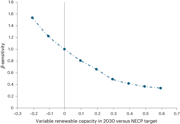
The figure represents the relationship between β-sensitivity of electricity prices and renewable capacity by 2030. The vertical axis represents the European average β-sensitivity, which measures the expected increase in the annual price of electricity when the price of natural gas increases by 1 euro. The horizontal axis represents the per cent over- or underachievement of the indicative targets for wind and solar PV capacity in the National Energy and Climate Plans of all Member States (plus ERAA forecasts for United Kingdom and Switzerland). For example, 20% means that the simulated variable renewable capacity is 20% higher in each country than envisioned in the NECP targets.

Source data

Full size image

Table 3 also shows remarkable differences across countries; looking at the European average does not tell the whole story. At +30% deployment of solar PV and wind, countries such as Italy or Austria would not achieve a β lower than 0.5, whereas Spain, Portugal and the Nordics would already be below 0.25. Achieving a β of 0.25 consistently across most markets in Europe would require between 50% and 60% of additional deployment. Note that the scenarios refer to simultaneous overachievement of national targets by all countries. In other words, it is necessary for every country to deliver over the target by 50–60%.

The differences in β-sensitivity across countries can be driven by several factors, including among others the availability of coal capacity and interconnection capacities. Given the highly nonlinear nature of market equilibrium in power markets, a full explanation is beyond the scope of this paper and is a relevant area for future research. However, one key factor to achieve a low β-sensitivity stands out: a higher number of hours where variable renewables set the price of electricity at their own, almost zero, variable costs.

An important implication of this result, as shown in Fig. 3, is that private, strictly market-based financing of much higher amounts of renewable capacity beyond the current 2030 targets could be very difficult under the current market rules in situations where β-sensitivity was very low. The reason for this is that the revenue of electricity sold by these technologies (that is, their captured price if selling directly in the day-ahead market) would be depressed as excess capacity would drive down prices during sunny and/or windy hours where they operate. Deployment at this scale would generate large curtailment of renewable electricity, which depresses revenues for all market participants and would have important implications for system stability²³. The saturation or cannibalization^24,25 of the price implies fewer opportunities to recover capital costs for renewable technologies if they are financed exclusively through their day-ahead market electricity sales. The larger the reduction in the sensitivity, the larger the resulting potential gap in the revenue of renewable plants. At the same time, prices of long-term contracts would be indirectly linked with short-term prices and expectations around them, the credit risk associated with buyers of Power Purchase Agreements (PPAs) or the policy reversal risk of contracts for differences (CFDs) would also depend on the variability of short-term prices, and in practical conditions, the overall supply of long-term contracts would still be conditioned by the volatility of natural gas prices. Hence, besides the logistical difficulties in achieving deployments 30% to 60% higher than the original NECP target by 2030, the financial viability of such deployment without policy support or other reforms is far from evident.

Average price at which wind onshore generators would sell their production (in the x axis) and the corresponding β-sensitivity parameter (in the y axis). Each point in the graph corresponds to a country and an assumed increase in renewable deployment. The renewable deployment scenarios are the same as those described in Table 3.

Source data

Full size image

We must stress that the results in Fig. 3 are constructed for the hypothetical scenarios where additional capacity is only added to solar PV and wind technologies. An important research question is whether other options to increase renewable capacity, for example, with different combinations of technologies, or including additional storage or improving interconnections, could achieve low β-sensitivity more effectively and generate market revenue that would make them investable without policy support. To obtain some insight into this question, we estimated results when storage capacity is deployed jointly with the new variable renewable capacity (Supplementary Section 7). These still find a strong positive correlation between β-sensitivity and captured price, which we attribute to the fact that the estimates maintain the projected natural gas capacity in 2030 unaltered, hence limiting the amount of additional storage that can be added profitably. In any event, future analysis (particularly in the context of the design of support mechanisms for renewables) should consider a broader range of deployment possibilities and explicitly evaluate their influence on the β-sensitivity parameters of the EU electricity markets.

Our results confirm that additional investments in renewable capacity in the European Union would be expected to lead to a large reduction in the volatility of electricity prices and their sensitivity to fossil fuel prices. The question is then to which extent this stabilization would have societal value in itself, that is, whether there is an insurance value of renewable investments as claimed by recent policy programmes.

Formally, the insurance value of an increase in renewables is the gain of welfare associated with the stabilization of consumption enabled by an increase in renewables due to their impact on power price stabilization, among other possible mechanisms. The underlying assumption is that some form of social welfare function can account for the societal value of uncertain future consumption streams. Risk aversion implies that social welfare is reduced by an amount ω because of the variability of aggregate consumption, compared with a situation with stable consumption over time with the same expected value. This formulation faces several controversies, including particularly on the choice of the discount rate and its adequate calibration to reflect risk aversion and income uncertainty²⁶ given equity premiums and other empirical evidence. Recent research tends to find that contrary to Lucas’ argument, economic volatility has large welfare costs^27,28, so that the value of economic stabilization policies is high. Therefore, the main question in our context must be whether deploying more renewables can be effective in stabilizing income and consumption at the aggregate level.

In Methods, we show that the effectiveness of additional renewables in stabilization is actually higher, among other factors, when it leads to a more intense reduction in the volatility and sensitivity of electricity prices to fuel prices holding the variance of the later constant. This is precisely the calculation we performed in the previous sections (Table 3), and the results there indicate that scenarios with large increases in renewables would result in very relevant reductions in both parameters. Whereas we do not quantify the insurance value of renewables fully in this paper, the results in Table 3 would support the view that there is in fact an insurance value of renewables and that it can be potentially large.

Whether it justifies different types or levels of policy support depends on the extent to which private investors do not consider the overall economic stabilization impact of their renewable projects. If they do not factor the insurance value, investment in renewables would be below the societal optimum even if their full environmental benefits were accounted for, for example, through a carbon tax. The idea that there may be an economic stabilization premium of some forms of energy is not a new concept in energy economics: a long tradition of research has focused on calculating the security premium of domestic oil versus imports²⁹ and estimates of this premium include a component capturing the possibility that domestic oil production lowers the exposure of the economy to supply disruptions and the fact that the marginal buyer does not recognize this effect when choosing its imports. Our results indicate that a similar exercise for renewable investments is warranted and would be an important area for further research.

Overall, a realistic quantification of the effects of additional renewable energy deployment through its ability to shield economies from fossil fuel price shocks, when also considering weather and demand volatility, suggests large stabilizing effects on electricity prices. We find that the capacity expansion plans as envisioned in the NECPs would lead to a reduction of the β-sensitivity to natural gas prices from 1.4 euros to 1 euro, which, in turn, would lower the extremes in prices that could be expected in the future. However, we find that the resulting improvement falls short of what would be required if the policy goal is to be close to independence from the prices of natural gas. Reducing the β-sensitivity to less than 0.5 euros would require deploying 30% more renewables by 2030, and going below 0.25 euros would require 60% additional deployment versus the currently envisioned target. These are very large changes. Moreover, further increasing the capacity of renewable technologies, while lowering the sensitivity and improving the stability of electricity prices, results in cannibalization conditions that would be associated with low market revenue for renewable producers in day-ahead markets. Hence, the financial viability of private investments based strictly on this market for reaching the capacity levels required to stabilize electricity prices is doubtful.

This is an important insight for ongoing debates on electricity market reforms in the European Union. Proponents of reform argue that the current design of markets in the European Union is not fit for the task of accommodating very high shares of renewables. The uniform-price auction or pay as clear nature of price setting in day-ahead European electricity markets, coupled with strong restrictions on capacity markets as sources of revenue for power plants, has been a hotly debated issue³⁰. In this design, the marginal costs of the most expensive plants required to satisfy demand set the price for all transactions in the market. Critics of the current design argue that this feature gives a disproportionate role to fossil fuel prices, and particularly natural gas, in the determination of electricity prices and impedes consumers from fully capturing the benefits of additional renewable power generation³¹. Those who defend the current market design argue, however, that setting prices at the costs of the marginal producers provides the right incentives to cheaper technologies to enter the market at the efficient level, avoiding the pitfalls of systems where capacity decisions are taken with a strong degree of administrative intervention^32,33.

In this regard, the most recent reform of electricity markets in Europe⁶ maintain the essential elements of day-ahead markets, while including support measures for long-term PPAs and a requisite to use CFDs in support mechanisms for new renewable capacity³⁴. If the objective is to use high renewable electricity capacity to reduce the sensitivity to natural gas prices, this implies depressing the prices achieved by renewable producers. Because the characteristics contemplated in these reforms make them mostly a risk-management instrument³⁵, the underlying financial viability of very large amounts of renewables would not be substantially improved by fair-valued CFDs.

Capacity mechanisms have also been proposed as part of these reforms, but recent literature has argued that they tend to favour technologies with higher fuel costs, rather than high capital cost options such as nuclear³⁶. In these conditions, capacity mechanisms would favour technologies that increase price volatility. Our results suggest that this side effect is very relevant and open the possibility that capacity mechanisms without further improvements in the availability of risk trading instruments could offset the price stabilization gains of renewable penetration.

Finally, the electricity price stabilization effect we document provides preliminary support to the notion that investment in renewables can reduce macroeconomic volatility. This in turn suggests that the insurance value of renewables, their ability to improve social welfare through their smoothing of economic shocks, could be substantial. This does not mean that power price stability is a goal in itself, to be attained regardless of the cost. But policy planning that focuses only on average magnitudes such as expected total system costs could be biased against renewables by failing to acknowledge the insurance value of renewables (or alternatively, the risk premium associated with fossil fuel technologies). However, as of today, none of the most relevant energy planning procedures in the European Union explicitly contemplate the power price stability contribution of renewables. It is not currently considered in the elaboration of the European Union’s National Energy and Climate Plans nor in the European Resource Adequacy Assessment. Our results provide a justification to advance in the potential integration of the insurance value of renewables in the social cost–benefit analysis of renewable investments and the institutional design of EU policies, and the concepts we advance could be applicable to other jurisdictions.

Expected changes in European markets generation capacity

We start by comparing the capacity plans for 2030 with the current capacity mix. For 2030, we take the power generation capacity targets by technology published in the EU member states’ National Energy and Climate Plans (NECPs). Introduced by Regulation (EU) 2018/1999 in 2018^37,38, the NECPs are the main long-term planning instrument for member states’ energy systems. The NECPs set out each country’s objectives for power generation capacity by technology within the Energy Union³⁹. Data for the United Kingdom and Switzerland are from the European Resource Adequacy Assessment¹⁸ (ERAA).

The NECPs anticipate dramatic changes in the installed generation capacity of European countries (Supplementary Section 2). We use 2024 as the reference year for the current capacity mix because this allows us to acknowledge generation capacity that is very close to coming into market or to closing. Countries’ plans foresee the doubling of variable renewables (wind and solar) from slightly above 500 GW to more than 1000 GW by 2030. Solar PV would experience the largest absolute growth, with the addition of more than 300 GW in this decade, whereas wind turbine capacity would increase by more than 230 GW (Supplementary Section 2 provides details). The plans also envision additions to hydropower capacity, battery storage and demand-side response, but on a much smaller scale. As for the retirements, all fossil fuel technologies experience reductions in capacity by 2030 in the NECPs, with coal being the most affected—capacity would be reduced by 41 GW, so that by 2030 coal power plant capacity would be approximately halved. The closure plans of nuclear plants in several countries would also lead to a sharp reduction total deployed capacity in this technology by 2030. Whereas there are important differences in scale across countries, the broad trend towards substitution of fossil fuels and nuclear with variable renewables is common to all countries. The NECPs also reflect a large expansion in the interconnection capabilities of European markets, which is also a driving factor of price formation. All interconnector projects in NECPs and the ERAA have been modelled (Supplementary Section 3).

Data sources

We use the databases representing the NECPs that were implemented as part of the ERAA¹⁸ of 2022 by ENTSO-E, the European Network of Transmission System Operators for Electricity. ERAA figures also include power generation capacity objectives for 2030 for two non-EU countries (the United Kingdom and Switzerland). The initial set of NECPs covering the period from 2021 to 2030 were submitted by countries in 2019. A revision of these initial plans was ongoing at the time of writing this article, but it was not possible to include the new information here as commission recommendations were issued only in December 2023 and several countries presented their plans with a delay.

The input data for the analysis are obtained from the 2022 ENTSO-E ERAA databases⁴⁰. The ERAA scenarios are based on the submission of countries NECPs, updated to account for recent trends and new information available after their publication. ERAA methodological document⁴¹ provides details on the statistical techniques and assumptions used by ENTSO-E to derive each database, including how climate years are considered, the treatment of electric vehicles and heat pumps and so on. Data in the ERAA databases are for each of Europe’s bidding zones. Supplementary Section 1 contains further detail on the data sources and their treatment.

Monte Carlo simulation design

Our simulation approach is based on creating a large number of future scenarios in a way that replicates the historical variability of weather conditions, demand fluctuations and the prices of fossil fuels. We use 300 future scenarios (that is, repetitions) in the analysis.

We replicate demand and fuel prices variability as follows. The initial data include 21 annual demand data series and four annual series for fossil fuel prices (natural gas, coal, oil and uranium). All of them are for the period between 1990 and 2021. We detrend each of these series (after taking logs) using a Hodrick–Prescott filter⁴² with lambda set to 100, following the standard approach for annual frequency data. This procedure results in 25 residual series: each of them can be interpreted as the (percentual) deviation from the respective series trend. By construction, these residuals have zero or close to zero average. We compute the variance and covariance matrix of these series: the components of this matrix capture the covariance between each of the 21 country/areas and the covariance of each of them with each of the four fossil fuel prices. Elements along the diagonal capture the variances of each of the 25 series.

Note that we keep CO₂ prices constant in the simulations as we consider them a policy variable, which can be adjusted by modifying the parameters of the ETS allowances allocation, as the European Union authorities have done systematically in the last decades.

We randomly draw 300 repetitions from a normal multivariate distribution with this same variance/covariance structure and zero average. This procedure results in a set of 300 future deviation from trend scenarios for each country demand and each fuel price which, by construction, replicate the variance–covariance structure of national demands and fuel price. These shocks capture annual frequency variations, driven by macroeconomic factors.

An important feature of ERAA data is that hourly capacity factors, weekly hydro inflows and hourly demands are provided adjusted for different weather conditions, replicating those observed for each year between 1987 and 2016 (the last year for which data are available for every country in the sample). We take full benefit of this by simulating electricity markets for randomly generated weather years, hence accounting for the historical variability in weather and its impact on capacity factors of wind and solar PV, inflows for hydropower technologies and the demand for electricity. Each repetition is assigned a randomly selected weather year between 1987 and 2016, using a uniform distribution. The weather year defines both the capacity factors of renewables and hydro and the hourly demand of each country (both its total level and its hourly profile).

Each of the 300 repetitions is thus characterized by a randomly selected vector of annual national demand and price deviations from trends and a weather year. More specifically, each repetition is characterized by the following three factors.

First, a vector with the prices of gas, oil, coal and uranium, each of them constructed as the product of the central reference price (which comes from the ERAA scenario) and the randomly generated deviation from trend.

Second, a vector of hourly capacity factors for variable renewables and inflows into hydro generators, which is determined by the randomly selected weather year, for each country.

Third, a vector of hourly demand for each country, which is determined as the central scenario corresponding to that weather year (coming from ERAA), scaled up by the randomly generated deviation from trend.

This procedure means that capacity factors and demand (both its profile and its level) are correlated as would be warranted by weather variations, whereas demand levels and fossil fuel prices are also correlated as dictated by their historical covariance.

We construct the scenario configuration for each of these 300 repetitions as follows: (1) generation and interconnection capacities are set at the levels foreseen in the NECPs as updated by the ERAA exercise for the horizon year being considered (2024 or 2030). (2) Each country/area demand is the result of taking the central forecast in the NECPs/ERAA databases for the horizon year (2024 or 2030), adjusted to reflect the corresponding weather year (randomly selected between 1987 to 2016) plus the deviation from trend resulting from the random shock to demand simulated to replicate historical volatility in national demand from long-term trend. (3) Fuel prices for the simulated scenario-replication are the result of taking the central reference prices of the NECPs/ERAA exercise for the horizon year (2024 or 2030) plus the deviation from trend resulting from the random shock simulated to replicate historical volatility in fuel prices from their trend. Each of these repetitions is then used to simulate the outcome of day-ahead markets.

The results in Table 3 simulate the same exact 300 future scenarios for hypothetical changes in the capacity mix. These changes are calculated increasing (in 10% steps) the nominal capacity of solar PV and wind (onshore and offshore) technologies.

Market simulation

We use GenX, an open-source electricity resource capacity expansion model, to replicate market dispatch¹⁹. GenX is a highly configurable system, which allows for complex simulation of electricity markets, including the possibility of finding optimal (that is, cost minimizing) capacity expansion plans, the simulation of operating reserves, unit-commitment restrictions, environmental and subsidy policies, among others. Our code only uses GenX dispatch module as, in our approach, capacity is defined by the National Energy and Climate Plans of EU member states, and because our capacity figures are given for national aggregates (that is, not at plant-level), some of the model features are less relevant (unit commitment, for example).

The simulation of market dispatch is carried out using version 0.3.0 of GenX. The only modification to the open-source version of the GenX algorithm was the addition of CO₂ ETS costs to the variable costs of all fossil fuel technologies. The code required for this is also available via Github at https://github.com/DanielNavia1/GenX-CO2Tax.

Given the size of the problem, each repetition usually requires approximately 0.5 h to solve in a modern personal computer. Because there are 300 repetitions (each of them with different demand, prices, weather) and 11 capacity configurations (one for 2024, nine for the sensitivity scenarios as depicted in Table 3, and the 2030 target scenario is repeated twice), full execution of the simulations would require approximately 9.8 weeks if performed sequentially. To shorten this time, the simulations were carried out using the University of Cambridge High Performance Computing platform through the Cambridge Service for Data-Driven Discovery (CSD3). The repetitions were performed in parallel with each of them assigned to a node with six cores, and a maximum of 50 nodes were used in each point in time. With this configuration, solving all the repetitions required for the analysis required approximately half a day.

Given a fixed configuration of capacities for a set of zones (country/areas in our implementation) and transfer capacities across zones (interconnections in our implementation), GenX’s dispatch algorithm minimizes the total variable costs of satisfying each zone’s demand at each of the 8,760 h in the year. The variable costs of each technology include a non-fuel variable operating cost plus a fuel cost, which is defined in turn by the fuel price per thermal MWh and the thermal efficiency of each plant type. GenX allows for the simulation of storage technologies, including hydropower plants with reservoirs and/or pumping capabilities and batteries. Because the algorithm minimizes the total annual cost, the resulting solution assumes perfect foresight of hourly profiles for capacity factors, inflows and demands for the full year. Hence, batteries and reservoirs will be charged and discharged in the optimal dispatch solution provided by GenX at the times that minimize the total cost of electricity generation for the full year. GenX includes the possibility to curtail demand if the cost of satisfying it exceeds a pre-set value of loss load parameter (set at 3,000 euros in our analysis). GenX also allows for demand-side response capabilities, which allow to anticipate or delay certain loads at a cost. The full solution of GenX dispatch is characterized by hourly generation profiles for each technology in each country/area and the hourly electricity flows across countries/areas (given the restrictions imposed by network capabilities). The Lagrange multiplier associated with the increase of 1 MWh in demand for a given country at a given hour is also calculated. Any technology in the model can set the marginal price, including variable renewables, storage, interconnectors or demand-side response.

The practice in European electricity markets is to use a common coupling algorithm (PCR-Euphemia⁴³) which, every day, finds the combination of generation and demand bids that maximizes total surplus, setting prices using a pay as settled mechanism. Let d_i (y, h, p) be the electricity demanded by agent i in hour h of the year y for a price p, and let s_j (y, h, p) be the electricity injected to the grid by agent j, again specified for hour h of year y, at sale price p. Because the algorithm maximizes total surplus aggregate for all agents, the solution will yield the result of a competitive market where the settlement price equalizes aggregate demand and aggregate supply at that price. In other words, p* (y, h), is such that (sum _{i}{d}_{i}left(y,h,{p}^{* }right)=sum _{j}{s}_{j}left(y,h,{p}^{* }right)).

Under the assumption of perfect competition and perfect foresight for the full year, the dispatch outcome of GenX would maximize the total economic surplus of generators and buyers in the day-ahead markets, replicating the result of a competitive market coupled with Euphemia. The Lagrange multipliers obtained would match the pay as settled prices that would be set in this market. Hence, we take prices obtained from GenX dispatch as a simulation of the outcome that would be obtained in European day-ahead markets. We acknowledge that this is just an approximation because the trading strategies of market participants may deviate from perfect competition and the predictability of demand, weather and so on is not perfect. Economic theory would suggest that large deviations from the perfect competition and perfect information setting should be capped to the extent that market participants can learn rationally and there is the possibility of free entry. In any event, the perfect competition case which we analyse here must be considered as a benchmark.

It is important to emphasize that our results are based on country-level zones, where we aggregate all bidding zones within a country into one. For some of the smaller countries, we aggregate them into hypothetical regional zones. Hence, our results do not account for transmission restrictions within countries and across smaller countries. ERAA data would allow analyst to carry out the same analysis with the full set of bidding zones and transmission capacities, but the computational requirements of doing so would grow notably and make it unfeasible in the context of this paper. The impact of this simplification on the results shown in this paper is likely to be different for each bidding zone. In zones with high renewables and low transmission capacity, the probability that renewable power set the price of electricity would be larger than indicated in our results, hence these zones would be expected to have lower sensitivity to fuel prices than what we present. The reverse situation would occur in zones with low renewables and low transmission capacity. Whereas our results do not model balancing costs, these would also be expected to be higher for bidding zones with smaller grids and high renewable penetration. Additionally, we cannot model local node constraints and balancing costs derived from the variability of renewables⁴⁴.

Empirical distribution of price outcomes

For each of the 300 future scenarios–repetitions obtained, the GenX dispatch model is run. Because the solution of the model is intensive in computing capability, the University of Cambridge High Performance Computing Resources are used for this purpose. The result is a set of 300 full simulations of the hourly market clearing outcomes in the future horizon year (2024 and 2030), where all repetitions share the same capacity configuration (including the network capabilities) but differ in the national demands, the fuel prices and the weather conditions being simulated.

We introduce here a stochastic characterization of electricity prices and their annual averages. The objective is to provide a mathematically solid foundation to our proposed measures of the instability of electricity prices.

Let y denote a vector summarizing the demand, fuel price and weather conditions prevailing in an electricity market in future scenario. Let p* (y, h) be the equilibrium price set at a bidding area at hour h for those conditions. Given K_Y, the capacity mix being analysed on the horizon year Y, over the 8,760 h of a year, the GenX algorithm yields a corresponding number of hourly equilibrium prices for each bidding area. From these, P(y), the annual price of year y is defined as the arithmetic average of hourly prices in the year:

We are interested in the stochastic properties of the conditional distribution (Fleft(Pleft(;yright)|{K}_{y}={K}_{Y}right)). Mathematically, we seek to understand how different measures of instability of annual electricity prices would evolve for different values of K_Y. Research has covered the variance, skewness and kurtosis of hourly, daily or weekly prices^5,9,10,45,46. These characterizations of hourly prices are key for several uses, including the operation of batteries or the charging of electric vehicles⁴⁵.

As explained, for each capacity configuration, we obtain 300 different scenarios (that is, 300 repetitions of y), which provide an empirical counterpart to the stochastic distribution (Fleft(Pleft(yright),|,{K}_{y}={K}_{Y}right)). Our results are based on the analysis of the empirical distribution so obtained.

Measures of volatility

The analysis in this article focuses on three key measures: annual volatility, percentiles of annual prices and the sensitivity to gas prices. Throughout, we use the subindex K to indicate that the measures of electricity price are to be derived from the conditional distribution given capacity, as explained in the previous paragraph.

Annual volatility (σ) is the standard deviation of the annual average price. This is the common definition of volatility for a stochastic variable.

Percentiles of the distribution of the annual price (pctile(K)). The standard deviation measure is a very partial description of the variability of the annual price, for two reasons. First, if the concern is with the probability of annual prices being very high, this parameter depends both on the standard deviation and the expected value of the annual price. Increasing shares of renewables may (in fact, are expected to) lower the expected price of electricity, so that a higher σ does not necessarily mean a higher probability of extreme prices. Second, the distribution of annual prices are expected to diverge from the normal distribution, even under the assumption that the joint distribution of demand and fossil fuel prices is normal. The estimates of the distribution obtained with the procedures in this paper reject the null hypothesis of normality in all but two countries, with clear indications that price distributions become bimodal in some cases (Supplementary Section 4) and a tendency for positive skewness. In view of this, we use the percentiles of the distribution of the annual price on Table 2. We use the 85th percentile as a reference for high but reasonably frequent prices and the 95th percentile as the reference for extremely high but very infrequent prices.

β-sensitivity (β(K)): note that neither the volatility nor the percentile measures can gauge the influence of natural gas prices on electricity prices. To measure this, we propose β the linear sensitivity of the annual price of electricity to changes in the price of natural gas. β is derived from the linear projection of the average annual price on the price of gas and other control variables X.

where ({L}_{K}left(Pleft(;yright),|,{P}_{mathrm{gas}},Xright)) denotes the linear projector operator. For each country and capacity configuration, we estimate the β-sensitivity with a regression of the observed annual price of electricity to the price of natural gas, and the only control variable we include is the price of coal. Regarding the choice of control variables, we only include the price of gas and coal because they make the interpretation of β-sensitivity more intuitive. Suppose that we added, for example, demand variables as a regressor. Then, the interpretation of a β-sensitivity of 1 would be that a 1 euro increase in the price of natural gas, holding demand factors constant, would be projected to lead to a 1 euro increase in the price of electricity. However, natural gas prices and aggregate activity are clearly related in Europe, and hence a shock to gas prices would lead to a reduction in energy demand, including electricity. Because we only include the price of natural gas in the regression, we can think about our estimates as best linear projections: that is, they would reflect the joint impact of natural gas both through the market clearing in electricity markets and their knock-on effect on aggregate demand. A β-sensitivity of 1 means that one euro increase in the price of natural gas would give a best projection on the price of electricity that is one euro lower, both because of the direct effect on market clearing and its correlation with demand. Note also that given the variability of annual prices due to other factors (weather, demand) in the simulation, the estimates of β-sensitivity are subject to sampling error. This explains that the estimated coefficient may be negative in some countries, where the actual true value would be 0 or close to 0. Supplementary Section 5 provides further clarification on the properties of β-sensitivity.

Relation between power price volatility and insurance value of renewables

Consider the following idealized model for electricity price formation whereby changes in the price of electricity relative to their average are a linear function of changes in fossil fuel prices (Δp_f), the component of seasonally adjusted electricity demand (d), weather conditions (w) and other random factors (u).

For simplicity, in this model Δp_f, d, λ w, e are assumed to be uncorrelated, so that the variance of electricity price (changes) is just the contribution of the variability of fuels and the variability of weather, in both cases considering the sensitivity to each of these factors, plus the variability of the other, unspecified, factors. Note that in our simulations we do not assume this: in our Monte Carlo design the correlation between fossil fuel prices and demand replicates their covariation in the period 1990 to 2021. Even holding the volatility of fossil fuel prices constant, additional investment in renewable capacity (which we denote by k_res) gives rise to countervailing effects as shown in equation (2):

On the one hand, renewables can potentially reduce the variability of electricity prices—and the likelihood of protracted spikes in electricity prices, such as those observed in 2022—as they lower the sensitivity of power prices to future shocks in the prices of fossil fuels (lower β). However, at the same time, systems with higher renewable capacity may be more exposed to fluctuations in demand and weather conditions (higher ψ and λ). Our simulation design allows us to obtain ({left.frac{mathrm{d}{{{sigma }}}_{{mathrm{pe}}}^{2}}{mathrm{d}{k}_{mathrm{res}}}right|}_{{sigma }_{mathrm{pf}}=mathrm{constant}}), that is, the change in the variance of electricity prices (Table 1 in the main text), and hence provide a quantification of which of the countervailing effects prevails. Moreover, whereas in this framework, we will use variance as the key statistic affecting the insurance value, in more sophisticated formulations it would be possible to use other statistics describing the distribution of electricity prices, including extreme values and the β-sensitivity. Our simulation design also produces estimates of these values (Tables 2 and 3).

We now show how the estimates of the changes in these parameters would feed into the calculation of the societal value of renewables attributable to their smoothing of economic volatility. The starting point is a representation of societal preferences over uncertain future consumption paths {C_t} that admits a representation in terms of the expected discounted value of the values of an instantaneous utility function u(), using a discount factor θ. The societal lifetime utility of an uncertain consumption path is then given by ({E}_{0}left[{sum }_{0}^{infty }{theta }^{t}u({C}_mathrm{t})right]).

Let (bar{{C}_mathrm{t}}={E}_{0}left[{C}_mathrm{t}right]) so that ({sum }_{0}^{infty }{theta }^{t}u(bar{{C}_mathrm{t}})) is the lifetime societal utility of a stable, certain path in which consumption at each period matches the expected value of the uncertain consumption path. The annual cost of economic variability ω is the amount that would need to be subtracted to the certain consumption path at every period so that its utility would match that of the uncertain path:

If u() represents the preferences of a risk-averse society, it must be true that ω is a positive quantity. In other words, society is worse off by an amount equivalent to ω every year because it gets the uncertain path, compared to a situation where it would get with certainty the expected value of consumption.

The insurance value of an increase in renewables is the reduction of this cost of uncertainty when renewables increase: (frac{mathrm{d}omega }{mathrm{d}{k}_{mathrm{res}}}). A useful way to characterize the insurance value of renewables is to decompose it as follows:

where (frac{mathrm{d}omega }{mathrm{d}{sigma }_mathrm{c}^{2}}) is the general value of stabilization (that is, the welfare gain associated with a less volatile consumption path) and (frac{mathrm{d}{sigma }_mathrm{c}^{2}}{mathrm{d}{k}_{mathrm{res}}}) is the stabilization of consumption achieved through renewable investment. As discussed in the main section of the paper, the higher the value of stabilization and the higher the stabilization achieved by renewables, the higher the insurance value of renewables. The discussion on the value of stabilization started with Lucas scepticism, but recent evidence points to large effects of economic fluctuations on societal welfare. This is consistent with the prevalence of stabilization policies in the fiscal and monetary realms.

We now turn to showing the relationship between ({left.frac{mathrm{d}{{{sigma }}}_{{rm{pe}}}^{2}}{mathrm{d}{k}_{mathrm{res}}}right|}_{{sigma }_{mathrm{pf}}=mathrm{constant}}), the parameter we estimate, and (frac{mathrm{d}{sigma }_mathrm{c}^{2}}{mathrm{d}{k}_{mathrm{res}}}) and (frac{mathrm{d}omega }{mathrm{d}{sigma }_mathrm{c}^{2}}). Consider a situation where consumption at time t is driven by the price of fuels and the price of electricity, together with other factors (unspecified but assumed unrelated with energy), for example:

This specification recognizes that what matters for aggregate outcomes is the price of energy, not only of electricity, and that different forms of energy can have different impacts. Fossil fuels are used in the economy for purposes other than electricity generation. In a social welfare analysis, the general equilibrium effects of increased renewable investment cannot be neglected. Hence, a change in the variance of consumption associated with faster renewable deployment impacts macroeconomic volatility not only through its effect on the β of electricity prices to fuel prices and the sensitivity to weather and demand, but also through the change in the relevance of fossil fuels’ and electricity prices in aggregate fluctuations (γ_f and γ_e, respectively) and the change in the volatility of fossil fuel prices. For simplicity, we maintain the assumption that Δp_f, d, λ w, u and ({rm{epsilon }}) are uncorrelated, which implies that the variance ({sigma }_mathrm{c}^{2}) is the weighted sum of their variances with appropriate weights derived in a straightforward fashion from β, ψ, λ, γ_e and γ_f. Differentiation of ({sigma }_mathrm{c}^{2}) with respect to k_res yields the following expression:

This expression confirms that the insurance value of renewables increases, the greater the reduction in the volatility of electricity prices due to investment in renewables, that is, as ({left.frac{mathrm{d}{sigma }_{mathrm{pe}}^{2}}{mathrm{d}{k}_{mathrm{res}}}right|}_{{sigma }_{mathrm{pf}}^{2}=mathrm{constant}}) is more negative. Coupled with the results in the literature on stabilization policies^27,28, our finding of comparatively large reductions in the variability of electricity prices would suggest a large insurance value. Note, however, that other general equilibrium effects of renewable investments would need to be considered too. These could occur through changes in the respective influence of electricity prices and fuel prices in the economy (the second term in equation (11)). Presumably, as long as the volatility of electricity prices remained lower than that of fossil fuels’ prices (recall this is annual frequency data), a shift towards electrification would increase the insurance value of renewables through this effect too. However, the impact of additional renewable investment on the volatility of fuel prices is itself a key consideration (namely, the third term in equation (11)). It might occur that additional renewables, by lowering the demand for fossil fuels and triggering unstable equilibria in their markets, could increase the volatility of fuel prices. These effects, if material, would tend to offset the insurance value of renewables.