Predicting debris flow pathways using volume-based thresholds for effective risk assessment

Introduction
Debris flow run-out and the associated risks to downstream population are important topics of research1,2,3. Usually, debris flow has long run-out within which most of the damage is confined, as the immense kinetic energy of debris destroys almost everything in its path4,5. Long run-out debris flows are common in tropical areas with high relative relief, such as in the Western Ghats. This area at the passive continental margin bordering the western coastal region of India is selected for this study (Fig. 1a). To our knowledge, the only physics-based susceptibility model for this region, developed by Sajinkumar and Oommen6, focuses solely on the initiation area, leaving the run-out zone unaddressed7. Their analysis of debris flow run-outs shows that these flows often traverse different landslide susceptibility zones (Fig. 1b). While debris flow initiation typically occurs in high-susceptibility areas, the run-out can extend into zones of moderate or low susceptibility, or even into areas considered non-susceptible. This creates a significant challenge for planners, as residents may feel a false sense of security in low susceptibility zones, unaware of the unpredictable nature of debris flow paths. Accurately predicting debris flow run-out, which is influenced by multiple factors, is therefore crucial. Landslide runout modelling helps in assessing the hazard and risk of fast-moving debris flows, and it can predict the dynamics of flow1,8,9. This study investigates 66 debris flows in the Western Ghats using comprehensive evaluation and modeling techniques. The goal is to understand the run-out dynamics of debris flows, which will aid in planning and developmental activities without the need for complex run-out modelling.

a Landslide inventory of Kerala for the 2018 storm event. It represents 4728 landslides where red represents the commonest type- debris flow, blue is shallow slide, and green is rock fall. b The catastrophic debris flow at Pettimudi in the Western Ghats overlaid with the Geographic Information System Tool for Infinite Slope Stability Analysis (GIS-TISSA) susceptibility map. The initiation of the flow was in the high susceptible zone but the run-out occupied even the medium and low susceptible zones. c Pancharakolli debris flow in Wayanad district, which followed the stream channel (SC-type). d Kattippara debris flow in Malappuram district, following a steepest hillslope (SH-type). The mismatch between the original and derived streams could be due to the low-resolution of the freely available elevation data (Image source: Google Earth; Software used for stream extraction (c, d): ArcGIS 10.2).
Study area
The western flank of the Western Ghats is susceptible to landslides due to its steep topography and weather pattern10,11,12. The area is directly exposed to southwest (June-September) and northeast (October–November) monsoons. High population density in landslide prone areas increases the vulnerability of the community to these natural disasters13, and parts of the Western Ghats within Kerala have a high population density averaging 859 persons/sq. km14. The Western Ghats experiences numerous debris flows each year during the southwest monsoon season. One exceptionally severe event of 2018, comprised of 2816 debris flows, 1760 shallow slides, and 152 rock falls15,16 (Fig. 1a). This event was the most devastating in recent memory17,18,19. The subsequent years also have witnessed catastrophic debris flows that killed hundreds of people at Kavalappara (2019; 59 deaths), Puthumala (2019; 17), Pettimudy (2020; 70), Kokkayar (2021; 7), Plappally (2021; 4), Kavali (2021; 6)10, and Wayanad (2024; ~250). For this study, we have selected 66 debris flows (Supplementary Fig. 1) across the state of Kerala with large area coverage i.e., more than 24,000 sq. m. These landslides demonstrate the unpredictable nature of landslide susceptibility zones, with significant casualties and destruction occurring even in low and non-susceptible areas. The events underscore the urgent need for comprehensive risk mapping that includes predicted run-out paths to enhance disaster preparedness and mitigate future losses.
Results and discussion
Debris flow run-out path
Debris flow will ultimately come to rest in one of two locations: either the nearest valley occupied by a body of water or a nearby plain. Theoretical models indicate that debris flows may follow one of the two possible paths: along the flow direction (SC), which can be a lower-order stream or along the shortest distance (SH), which corresponds to the steepest slope (Fig. 1c, d). Of the 66 debris flows, 60 followed SC, and six preferred SH (Supplementary Fig. 2). This was identified by comparing the run-out with the interpreted drainage network.
Calibration of rheological parameters
To match the volume with the areal extent for each of these 66 debris flows, a trial-and-error approach was employed. Figure 2a, b presents the results for two representative debris flows, one following the SC path and the other following the SH path, and illustrates the increase in length and width that accompanies increasing release volume. The dry-Coulomb type friction controls the final flow characteristics when the flow is slow20, with high values reducing the run-out length (Fig. 2c, d). On the other hand, viscous-turbulent friction controls the flow when the materials flow at high velocities, as shown in Fig. 2e, f. The obtained best-fit values were used to get the run-out parameters such as flow height, velocity, pressure, and deposition (Fig. 2g–n). During the initial stages of a debris flow, flow height, velocity, and pressure tend to be highest, typically occurring in the areas characterized by higher susceptibility classes characterized by steep slopes. However, deposition tends to occur in areas where the slope is less pronounced and susceptibility is low.
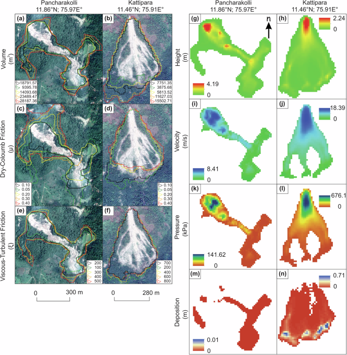
Trial and error method using RAMMS adopted to calibrate release volume (a, b), dry-Coulomb type friction (c, d) and viscous-turbulent friction (e, f) for Pancharakolli and Kattippara debris flow. The best fit simulation is shown in black. Increase in volume increases the area of the run-out. The dry-Coulomb type friction controls the rapid flow that is mainly in initial stage of flow whereas the viscous-turbulent friction controls the slow flow that is mainly concentrated at the zone of deposition. g–n The best-fit model for Pancharakolli and Kattippara debris flow where: Flow height (g, h), which helps in assessing the impact of landslide on buildings and other infrastructures; higher flow causes more damage. Flow velocity (i, j), where higher velocities are at high slopes and at the initiation zone; higher velocities have more energy and cause more damage. Flow pressure (k, l) exerted by debris flow; higher pressure are at initial stages and causes more damages. Height of materials deposited by debris flow (m, n) is mostly at the zone of accumulation where the slope is gentle; larger volume of deposition poses high threat to life and property (Image source (a–f): Google Earth; Software used (g–n): RAMMS::Debris Flow).
Accuracy of simulation
The accuracy of matching debris flow run-out simulation to actual debris flow footprint shows that the debris flow following SH can be well characterized. The simulation results cover more area than that of the actual debris flow due to constraints in the resolution of elevation data. An average of 93% area of SH-type was covered by simulation, whereas for SC-type the coverage was 82%. The modelled debris flow and real debris flow footprint were intersected, and the average area matching was 53% for SH-type and 32% for SC-type. The excess area simulated by the model over the real condition is 40% for SH-type and 62% for SC (Fig. 3a–d). The SC debris flows have lower release volume than SH-type, but their narrow and long run-out path is due to the pre-existing channel morphology and pore-water pressure. This long narrow run-out simulated with a medium-resolution elevation data tends to occupy wider paths than actual, which led to excess area.
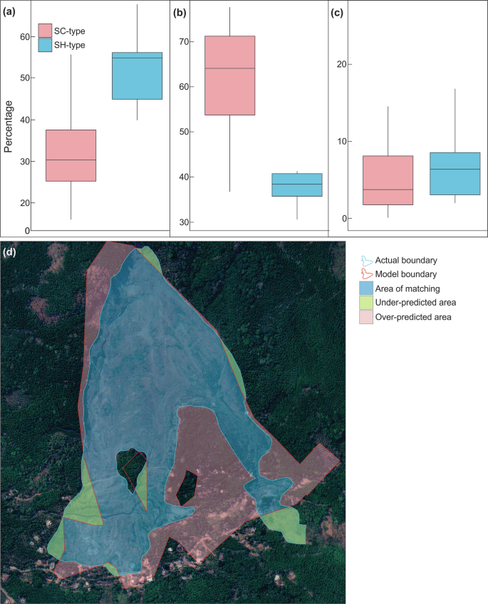
The accuracy of simulated debris flow to the real-world condition. a The percentage of area of true positive, SH-type is well matched with real world scenario. b The percentage of area of over prediction. High over prediction in SC-type debris flow and low in SH-type can be seen. c Under predicted area is very less for both SC-type and SH-type of debris flow. d Kavalappara debris flow in Malappuram district, Kerala overlaid with real debris flow area and area simulated (Image source (d): Google Earth; Software used (a–c): R and (d): RAMMS::Debris Flow).
Identifying the threshold
The flow path characteristic of a debris flow is controlled by run-out material and release volume, which is the initial energy source. The wider and shorter run-out paths for SH-type are due to high release volume, whereas longer and narrow run-out path for SC-type is due to existing channel and water content. The distribution of release volume and friction coefficients such as dry-Coulomb, and viscous-turbulent are shown in Fig. 4. Release volume is determined by estimating the release area and release depth from field observation, which, for this event, ranges between 901 and 93859 cu. m.
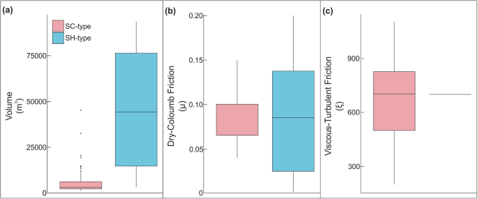
Control of volume, dry-Coulomb type friction and viscous-turbulent friction in determining the flow path of debris flow. a Debris flow with low release volume tend to follow flow direction and with high release tend to flow shortest distance. b Both type of debris flows have a wide range of dry-Coulomb type friction and cannot be divided based on dry-Coulomb type friction. c Viscous-turbulent friction has a wide range of values for SC-type following flow direction but narrow range for SH-type debris flow (Software used: R).
To derive the threshold for differentiating SC and SH debris flow types, an interquartile method was used. In this approach, the upper quartile (75th percentile, Q3) of SC and the lower quartile (25th percentile, Q1) of SH were analyzed to identify a potential threshold. The threshold was estimated as the midpoint of the gap between Q3 of SC and Q1 of SH (Fig. 5a). To assess the variability of this threshold, bootstrapping was applied by generating multiple resampled datasets with replacement. For each resampled dataset, the threshold (midpoint between Q3 of SC and Q1 of SH) was calculated, allowing a non-parametric confidence interval to be determined, which reflects the natural variability within the data sample. The bootstrapping results yield a median threshold of 7072 cu. m with a 95% confidence interval ranging from 3800.35 to 32322 cu. m. This median threshold serves as the central estimate from 20000 bootstrapped thresholds and is robust against skew or outliers, making it a reliable central measure. Figure 5b illustrates the probability density functions for SC and SH volumes, with the threshold and confidence interval visually displayed to highlight the overlap and uncertainty in classification. This plot highlights the overlap between SC and SH distributions, and shows the range where classification is uncertain due to data variability.
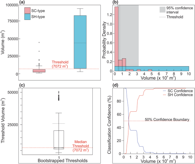
a Box Plot of SC and SH debris flow volumes with threshold line indicates the proposed division between SC and SH types, helping visualise the boundary based on typical volumes. b Histogram of SC and SH debris flow volumes with threshold and confidence interval. The histogram overlays the probability density functions (PDF) of SC and SH debris flow volumes. The median threshold of 7072 cu. m is marked with a vertical dotted line, while the shaded area represents the 95% confidence interval (3800.35 to 32322 cu. m). c Box Plot of Bootstrapped Thresholds with 95% Confidence Interval. The box plot represents the distribution of 20000 bootstrapped threshold values, with the median threshold at 7072 cu. m and a 95% confidence interval. d Classification confidence levels for SC and SH debris flow volumes. The line plot shows the classification confidence for SC and SH types as debris flow volume varies. Confidence levels decrease as volumes approach the threshold (7072 cu. m), where classification is less certain.
Figure 5c shows the distribution of bootstrapped threshold values, providing insight into the natural variability and reliability of the estimated threshold. Practically, debris flow volumes below this threshold are more likely to belong to the SC-type, while those above are likely to be SH. The wide confidence interval suggests that, while 7072 cu. m is the best estimate, the true threshold may vary between 3800.35 to 32322 cu. m due to inherent variability in the data. This broad interval indicates substantial variability or potential overlap between SC and SH distributions, which makes precise classification challenging. However, the 7072 cu. m threshold remains a practical and viable option, especially when used within a probabilistic framework. Lastly, Fig. 5d demonstrates the utility of a probabilistic framework, showing how classification confidence varies near the threshold. This approach enables flexible classification, with higher certainty for volumes significantly below or above the threshold and a probabilistic zone for volumes near it. With additional data, this method could be refined further, potentially narrowing the confidence interval and improving classification accuracy, enhancing its practical value in distinguishing between SC and SH debris flow types. If the initial release volume is less than 7072 cu. m, debris flow tends to follow SC; otherwise, it will be SH. In order to quantify the release volume of a given area, it is necessary to determine the thickness of the soil present in different susceptible regions. Although measuring soil thickness can be challenging, techniques are available to estimate this quantity based on slope measurements21,22. Meanwhile, the friction coefficients such as dry-Coulomb, and viscous-turbulent do not appear to exert significant control over the behavior of debris flow in this area, since there is no boundary for defining the threshold (Fig. 4b, c). The effect of these debris flows on deposition, velocity, pressure, and flow height are shown in Fig. 6a–d. Deposition of materials occurs in a gentle slope, which is normally non-susceptible. Deposition, velocity, pressure, and flow height are higher in SH-type. During rainstorm events, the surface runoff will be mixed with SC debris flows. In SH-type there is much less effect of water, and one would expect that the run-out will be shorter. But as the slope is steeper, the energy will be high, and thus, the velocity and pressure are high. These 66 debris flows cover an area of 7.93 sq. km. 76% of this area is occupied by 60 SC-type debris flow and 24% by six SH-type debris flows (Fig. 7). This is due to the huge volume of material released by SH-type that makes wider run-outs than SC-type debris flows with less volume. The trend of debris flow leading to catastrophic consequences on life and property is caused by deposition occurring outside the high susceptibility area than within it. The severity of this issue arises due to the perception of these areas as safe for habitation.
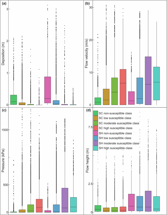
Analysis of run-out parameters in different slope stability classes. a Deposition of materials occurs in gentle slope, which is normally non-susceptible. The trend of deposition is inversely proportional to landslide susceptibility. Deposition is higher in SH-type debris flow. b Flow velocity increases with increase in landslide susceptibility due to increasing slope. Velocity is higher in SH-type debris flow. c Pressure of flow increases with increase in landslide susceptibility. Pressure is higher in SH-type debris flow. d SH-type debris flow has higher flow heights than SC-type (Software used: R).
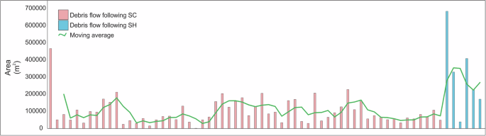
Run-out area of 66 debris flow. The pink colour represents the SC-type and blue shows SH-type. SH-type has high area coverage than SC-type. The green line shows the three-period moving average (Software used: R).
The results show that the release volume is crucial in determining the run-out path. The debris flow with a higher release volume than the threshold value (7072 cu. m) tends to follow SH-type. The high energy associated with the material volume might have caused high velocity for SH-type in contrast to SC-type that follows a flow direction path with low release volume. The high release volume makes SH debris flow more hazardous than SC. The threshold derived in this study to determine the path of debris flow can be used to classify them and assess their potential impacts on communities residing in areas with different susceptibility levels. Hence, this threshold can be employed to create landslide risk maps. The results of this study establish a threshold volume of 7072 cu. m to distinguish between SC and SH paths in debris flows. This threshold, based on RAMMS modeling of 66 debris flows in the Western Ghats, allows for predicting flow paths using only terrain data, such as digital elevation models (DEMs), rather than running computationally intensive simulations for each event. Although RAMMS simulations can predict flow paths accurately, our threshold provides a practical alternative, particularly valuable for local decision-makers who may lack expertise in specialized modeling software. By using this volume threshold, practitioners can quickly determine the likely flow path based only on debris volume, supporting cost-effective and timely risk assessment and planning. Thus, this threshold-based approach serves as a useful tool in hazard mitigation, enabling regions with limited resources to assess debris-flow dynamics and plan accordingly without extensive computational demands. However, the creation of such maps is beyond the scope of this study, and therefore warrants further research. Attempts to create susceptibility maps with run-out area were attempted earlier23, but its reliability in comparison with the existing susceptibility maps need to be validated in areas like the Western Ghats. Based on the outcomes, it should be noted that the RAMMS model exclusively takes into account the volume and material properties of the landslides and neglects other significant influencing factors. The simulation of the narrow run-out path for SC-type debris flow using 12.5 m elevation data is also challenging and caused over-prediction of debris flow area.
Methods
The run-out characteristics of catastrophic debris flows of the study area have been assessed using a computer program called Rapid Mass Movements Simulation (RAMMS)::Debris Flow. Previously, RAMMS has been successfully used for modeling the run-out scenarios of a few independent slides in the Western Ghats24,25. This computer program predicts the flow path, distance, and velocities based on slope, soil and depleting mass conditions26. The simulated output from the model predicts the slope-parallel velocities and flow heights using depth-averaged equations26. The model requires basic input parameters such as initial release volume and a digital elevation model (DEM). Two types of release information are available for use in the model: block release and hydrograph. We adopted the block release method in this study, as the data availability limits the use of the hydrograph model. The input DEM used is ALOS PALSAR with 12.5 m spatial resolution, which can be freely downloaded (www.asf.alaska.edu/). RAMMS uses the Voellmy-fluid friction model, which is controlled by two friction parameters: dry-Coulomb type friction (μ) that scales with normal stress, and a velocity-squared drag or viscous-turbulent friction (ξ)25,27. Dry-Coulomb type friction ranges between 0.01 and 0.2, and viscous-turbulent friction between 200 and 1100 m/s2. These rheological parameters are estimated through a trial and error approach such that the simulation best fits the debris flow footprint (observed best-fit was utilized) whereas the volume estimation is based on the soil thickness in the scarp area, given as input release depth (m) in RAMMS. This helps in identifying the drivers of each long run-out debris flow. The parameters used are given in Supplementary Table 1.
The drainage networks for the Western Ghats were derived from ALOS PALSAR elevation data using the hydrology tools in ArcGIS (https://desktop.arcgis.com/en/arcmap/). Drainage was derived from flow accumulation raster. A threshold for flow accumulation was derived by matching the drainages paths of the Survey of India topographic sheets on 1:25000 scale. Drainage pattern and debris flow run-out were compared to identify whether debris followed the existing stream channels (SC) or the steepest hill slope (SH). Slope stability classes derived using the physics-based GIS TISSA model28 were used to quantify the different susceptibility zones through which the run-out of these 66 debris flows navigated. The selected 66 debris flows range in length from 218 m to 5766 m with a mean length of 945 m and run-out area between 24,375 sq. m and 684,141 sq. m.
Based on the ALOS PALSAR topographic data and by varying the parameters such as the release volume and both the friction coefficients, a simulation was conducted. Initially, the simulation was setup with the default frictional parameters (μ = 0.2, ξ = 200 m/s2), and different release volumes. The results were checked for the degree of match and mismatch. Simulation was performed repeatedly with varying volumes and friction coefficients until an optimal match was reached as compared to the real conditions. The release depth was adjusted to cover the areal extent of the debris flow, whereas friction coefficients were adjusted to match the run-out. The release area was identified through field observations and then cross-referenced with high-resolution imageries from Google Earth. It is worth noting that the increase in the release depth leads to corresponding increase in both volume and run-out. The friction coefficients and the release volume information of the best matching simulation of 66 debris flows were analyzed to identify the threshold of these parameters that define the flow type. The schematic diagram of the methodology described above is shown in Supplementary Fig. 3.
: spatial distribution characteristics and implication for the seismogenic fault")

Responses