Probabilistic machine learning for battery health diagnostics and prognostics—review and perspectives

Lithium-ion (Li-ion) batteries have witnessed growing adoption in consumer electronics, electric vehicles (EVs), and grid energy storage systems, largely owing to their excellent energy density and power output. However, continued usage and adverse operating environment drive irreversible chemical reactions and material morphology changes, leading to gradual but inevitable degradation of battery capacity and power over time. Consequently, accurately estimating the state of health (SOH) of Li-ion batteries and predicting their future degradation is crucial to optimizing every part of the battery life cycle—from research and development, to manufacturing and validation, deployment in the field, and reuse and recycling¹.

Some of the earliest research into Li-ion battery health diagnostics and prognostics focusd on mathematical modeling of the capacity fade during cycle aging tests^2,3,4. Notably, Bloom et al.⁴ found that the cell capacity could be aptly captured by a modified Arrhenius relationship, which is generally used to describe the rate of a chemical reaction. This capacity fade model excelled in extrapolating battery performance to new, untested conditions, providing great utility for design and engineering. Not long after, researchers began experimenting with empirical and semi-empirical mathematical models for battery capacity fade modeling to gain better accuracy. In the work of Spotnitz⁵, researchers developed a semi-empirical model for Li-ion battery capacity fade considering reversible and irreversible capacity loss due to solid-electrolyte interphase (SEI) growth on the graphite anode in the cells. Similar work by Broussely et al.⁶ proposed an empirical quadratic equation to model the capacity fade of NMC/Gr Li-ion cells during long-term storage. The quadratic model was primarily developed to capture the effect of SEI growth from electrode-electrolyte reactions during storage. Later, Liaw et al.⁷ demonstrated that empirical models could be used to extrapolate cell resistance increase with thermal aging to update the parameters of a simple equivalent circuit model for capacity estimation. Since these initial seminal works, many more advanced empirical and semi-empirical models have been developed^8,9,10.

The great success of empirical and semi-empirical models soon led researchers to investigate alternative methods of modeling battery aging from experimental data. Saha et al.¹¹ were some of the first to use a machine learning (ML) algorithm as part of a framework to model battery capacity fade and predict remaining useful life. The researchers used a relevance vector machine (RVM) (see the section “Relevance vector machine”) to model the exponential growth observed in the cell’s internal resistance with aging. The RVM was used to predict future resistance parameters for an equivalent circuit model that was then used to predict cell capacity. Altogether, the RVM was shown to do an exceptional job at rejecting outliers from the dataset and providing good uncertainty estimates with its predictions. This approach inspired others to further investigate ways of using ML models for battery health diagnostics and prognostics^12,13,14.

Over the past decade, the use of ML for battery health diagnostics and prognostics has expanded substantially. The rapid growth can be attributed in part to the recent advances in ML and deep learning technology, like open-source ML software and datasets, that enable easier modeling of complex data¹⁵. Well-studied applications of ML for battery health diagnostics and prognostics include battery performance simulation and state estimation (primarily state-of-charge (SOC) and power estimation)^16,17,18,19, SOH estimation and capacity grading^20,21,22, and capacity forecasting and remaining useful life (RUL) prediction^23,24,25. Newer, emerging battery prognostic problems include early lifetime prediction^26,27, knee point prediction²⁸, capacity trajectory prediction from early aging data^29,30, and initial works investigating the applicability of existing diagnostic and prognostic models to battery aging data collected from the field^31,32,33.

Despite these significant research efforts on battery health diagnostics and prognostics, most ML-focused works have yet to incorporate uncertainty quantification systematically. Here, “uncertainty” refers to the predictive uncertainty of an ML model, such as a neural network, for a training/test sample point that is ideally associated with how confident the model is when predicting at this point³⁴. The idea is that an ML model does not simply produce an output (e.g., an estimate of a cell’s SOH indicator); it also estimates the uncertainty associated with this prediction to the most accurate extent possible. For example, this predictive uncertainty can be in the form of a standard deviation of a Gaussian-distributed output that describes the spread of the probability distribution around the mean prediction. A spread that is too large indicates that the uncertainty level is high enough for the output not to be trusted. In such cases, a human end user may discard this prediction or provide the ML model with additional information to reduce the predictive uncertainty. Predictive uncertainty can be confused with prediction error. The former comes as an uncertainty estimate by an ML model with uncertainty quantification capability and is thus known; in contrast, the latter is unknown without access to the ground truth. That is why access to predictive uncertainty is important for applications not tolerating large prediction errors well. Ideally, in these applications, we expect predictive uncertainty (known) to be a reliable indicator of prediction error (unknown) on a per-sample basis.

Quantifying predictive uncertainty in ML-based health diagnostics and prognostics becomes especially important given the dynamic and multi-physical nature of Li-ion batteries, where even small variations in manufacturing and testing conditions can significantly change the electrical, thermal, and mechanical performance, resulting in larger cell-to-cell variability³⁵. Furthermore, this inherent cell-to-cell variability becomes even more pronounced as the cells age. Early work by Baumhofer et al.³⁶ investigated the production-caused variation in capacity fade of a group of 48 cells cycled under identical conditions, finding that the lifetimes varied by as much as a few hundred cycles. These results, and many similar studies^26,32,35,37, highlight the great need for probabilistic diagnostic and prognostic algorithms that often have to learn from small datasets and extrapolate to the tail-end of the lifetime distribution for a population of cells. Such extrapolations are often associated with large prediction errors, which, although infeasible to quantify without access to the ground truth, can be communicated to the user, to some degree, through high predictive uncertainty and low model confidence. Probabilistic models with properly calibrated uncertainty estimation are paramount for setting warranties on battery-powered devices like consumer electronics and, more recently, EVs, where failing to deliver a promised lifetime due to maintenance/control decision making informed by largely incorrect ML-based diagnostic and prognostic results can cost companies their reputation in addition to the monetary burden associated with honoring warranty repairs.

In practice, quantifying diagnostic and prognostic uncertainty is especially important for large battery packs with many modules, where the capacity of a module consisting of serially connected cells will be limited to the capacity of the worst-performing cell. Thus, probabilistic models (like those discussed in the sections “Probabilistic ML techniques and their applications to battery health diagnostics and prognostics”, “Advanced topics in battery health diagnostics and prognostics”, and “Future trends and opportunities”) that can accurately model worst-cell performance through uncertainty estimates made by learning from a limited dataset are crucial to module and pack development. This cell-to-cell variability poses a direct challenge for battery management systems (BMSs) that need to balance cell voltages to maximize the capacity and power availability of a battery pack. In essence, a BMS is an electronic system consisting of hardware, software, and firmware that is responsible for managing the power and health of a rechargeable battery (e.g., a Li-ion battery cell or pack). Figure 1 outlines some key functions of a BMS in an illustrative flowchart. The BMS in the figure is built for a battery pack consisting of SE serially connected strings (or modules), each with PL parallelly connected cells. The BMS takes voltage (V), current (I), and temperature (T) measurements from each cell in the pack at regular intervals (e.g., every 1–5 s) and estimates the SOC and SOH of each cell, both of which cannot be directly measured. As will be detailed in the section “Battery health diagnostic and prognostic problems”, SOH estimation is an important battery diagnostic problem. For situations that require knowing how long each cell/module can be used before replacement, the BMS monitoring module also predicts each cell’s RUL and, in some cases, the cell’s SOH trajectory in future cycles. RUL prediction and SOH trajectory prediction are two well-studied battery prognostic problems of significance, as will be discussed in the section “Battery health diagnostic and prognostic problems”. Most importantly, neglecting uncertainty when predicting cell SOC and SOH may lead the BMS to incorrectly balance cell voltages, ultimately reducing the available capacity and power of the pack. It is worth mentioning that SOH estimation and RUL prediction can be computed in the cloud instead of directly at the BMS device, as the SOH and RUL usually need not be updated in real-time.

This battery pack comprises SE serially connected strings, each of which is composed of PL cells connected in parallel.

Full size image

One major advantage of predictive uncertainty quantification for battery maintenance and control is its value in informing BMS actions during operation. For example, if estimates of cell SOC are highly uncertain, the BMS may limit the overall charge power in order to prevent cells from entering over-voltage conditions during charging. However, parameterizing models that can accurately quantify predictive uncertainty is challenging because battery datasets are usually limited in size due to the large expenses required to operate thermal chambers for extended periods. Further, it is difficult to replicate real-world operating conditions in the laboratory, and much care is needed to ensure newly parameterized models can accurately quantify prediction uncertainty on field data (see the section “Diagnostics and prognostics using field data”). The trend of small datasets is likely to continue as cells grow larger in size for automotive and grid storage applications. Large-format and high-capacity (>100 Ah) Li-ion battery cells require even more expensive testing equipment to achieve the high C-rates (>3C for a 100 Ah cell requires >300 A continuous current) necessary for aging cells quickly and studying fast-charging protocols—research that is imperative for lowering the “refueling time” of today’s EVs and accelerating the transition to electrified transportation. With costs for cells and test equipment on the rise, calibrating the predictive accuracy and uncertainty of battery diagnostic and prognostic models prior to deployment becomes critically important. Incorrect control decisions based on erroneous predictions and uncertainty may lead to suboptimal performance, damage to battery cells, and in rare cases, thermal runaway that results in catastrophic product loss and endangers the safety of people nearby.

To this end, developing and validating probabilistic battery diagnostic and prognostic models is an essential area of research in the battery community. A handful of reviews on battery health diagnostics/prognostics exist today and can be found here^{38,39,40,41,42,43,44,45}. However, all the reviews to date focus primarily on deterministic ML modeling methods, and do not emphasize existing research that studies probabilistic methods for battery health diagnostics and prognostics. To address this gap, we seek to provide a comprehensive overview of probabilistic modeling and ML for battery health diagnostics and prognostics. After providing an overview of Li-ion battery degradation, we review past and present studies on probabilistic battery health diagnostics and prognostics and discuss their methods, advantages, and limitations in detail. Our review offers unique insights into each of the probabilistic modeling approaches with detailed discussions on the implementation approach and recommendations for future research and development. Figure 2 presents an outline of this review paper. Below are a few key items covered in our review.

1. 1.

   First, we provide an overview of Li-ion battery degradation, discussing the types, main causes, and resulting effects on cell-level performance and SOH in the sections “Battery degradation—modes and mechanisms” and “Battery state of health”. The classification of battery degradation modes and analysis of their root causes provides relevant background knowledge that motivates the need for battery diagnostic/prognostic models that can estimate cell health and predict future cell degradation. In the section “Battery health diagnostic and prognostic problems”, we provide a high-level overview of six general problems relevant to battery health estimation and life prediction. Additionally, we highlight the pivotal role that publicly available battery aging datasets have played in facilitating existing research in the area (the section “Publicly available battery aging datasets”).

2. 2.

   Second, we analyze and compare the advantages and limitations of various probabilistic ML techniques and their application to battery health diagnostics and prognostics (the section “RVM applications to battery diagnostics and prognostics SOH estimation”). This section, uniquely focusing on probabilistic techniques for health diagnostics and prognostics, covers both the methodologies of each technique and examples of its applications to SOH estimation, SOH forecasting, and RUL prediction. This particular emphasis on probabilistic ML is a noteworthy feature of this review that sets it apart from existing reviews on battery health diagnostics and prognostics.

3. 3.

   Third, we delve into three emerging and “newer” topics in battery health diagnostics and prognostics in the section “Advanced topics in battery health diagnostics and prognostics”. Specifically, this section offers unique insights from three researchers actively working on problems related to battery SOH estimation from field data (the section “Diagnostics and prognostics using field data”), degradation diagnostics (the section “Degradation diagnostics”), and early life and trajectory prediction (the section “Early life and trajectory prediction”). This unique coverage of emerging topics further sets our review apart from existing ones.

4. 4.

   Fourth and finally, we discuss future trends and research opportunities in physics-based prognostics (the section “Physics-based diagnostics and prognostics”), second-life applications for used Li-ion cells (the section “Second-life applications”), and aging-aware battery control optimization (the section “Aging-aware battery control optimization”). This discussion constitutes the final distinctive element of this review, not commonly found in most other reviews.

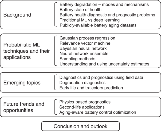
Outline of sections and subsections.

Full size image

Our review paper is concluded in the section “Conclusion”, where we also discuss prospects for future research essential to addressing long-standing challenges in battery health diagnostics and prognostics.

It is worth noting that this review focuses primarily on the application of various probabilistic ML and deep learning methods to unique problems (the section “Battery health diagnostic and prognostic problems”) within the field of battery health diagnostics and prognostics. A limitation of this work is that it does not cover specific challenges related to emerging ML topics, such as hybrid modeling, transfer learning, federated learning, and similar ML-focused concepts.

Battery degradation—modes and mechanisms

Battery degradation is a complex and multi-scale process that varies with cell design and is driven by the way a cell is used. Understanding the fundamental mechanisms of Li-ion battery degradation is essential for effectively modeling and designing around it. Typically, researchers and engineers will conduct lab-based aging experiments to study the effects of different operating conditions on cell aging and SOH, which is most often quantified as a cell’s remaining capacity or internal resistance. Periodic reference performance tests (RPTs) are carried out during aging experiments to assess cell capacity and resistance under standard conditions (usually 25 °C) to help isolate the effect of aging on changes in cell capacity and resistance⁴⁶. Comparing cell SOH measured from RPTs is important because cell capacity and resistance are influenced by temperature, C-rate, voltage limits, among other factors.

Battery aging tests are used to understand how stressors, like time, temperature, and energy throughput, affect the rate of capacity fade and the progression of internal degradation modes^47,48. An overview of battery degradation mechanisms, their corresponding modes, and measurable cell-level effects is shown in Fig. 3. Even without cycling, Li-ion batteries lose capacity over time as internal side reactions occur between the electrolyte and electrode materials. The most prevalent of these side reactions is the formation of the solid electrolyte interphase (SEI) on the graphite anode common in nearly all Li-ion batteries used today⁴⁹. SEI growth is mainly driven by time, but is also influenced by temperature, cell voltage, and cell load⁵⁰. Fortunately, the formation of SEI on graphite anodes is entirely expected and well-studied as it plays a large role in determining a battery’s maximum capacity and expected lifetime. It has been widely accepted that capacity fade from the growth of SEI scales with a square-root-of-time (Q(t) = a ⋅ t^0.5) relationship⁹. Further, many researchers have modeled Li-ion battery capacity fade due to SEI formation at various temperatures by scaling the t^0.5 term using Arrhenius-like equations that model the influence of temperature on reaction rate^51,52. Additionally, SEI formation has been shown to be directly related to the SOC a battery is stored at, where higher voltages generally lead to faster reactions and greater capacity fade. However, next-generation battery designs are pursuing new anode materials and may reduce or even eliminate the use of graphite in the anode altogether, thus introducing new degradation mechanisms that will need to be studied and mitigated.

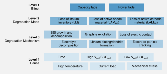
Figure modified from Thelen et al.⁸¹ and based on the original figure in Birkl et al.⁷¹ showing the relationship between cell use/environment (Level 4), the corresponding degradation mechanisms (Level 3), their connections to the degradation modes (Level 2), and the resulting capacity/power fade (Level 1).

Full size image

When a Li-ion battery is cycled, more degradation mechanisms arise in addition to the always-present capacity fade from SEI growth and other side reactions. Often during cycling, the SEI growth rate accelerates because the movement of Li-ions in/out of the electrodes causes repeated swelling and subsequently cracking of the already formed SEI, revealing new sites for SEI to form, and ultimately consuming more lithium in the process^51,53,54. Like SEI formation, electrode swelling is expected by battery designers, and is a well-studied degradation mode. Li-ion battery degradation from electrode cracking has been shown to be sensitive to the depth of discharge (DOD) and the C-rate the cell is subjected to—where deeper discharge and faster rates increase the rate of capacity fade^26,51,55. Capacity fade driven by electrode cracking during cycling has been diagnosed as a primary driver of cycling-driven capacity fade in Nickel-based battery chemistries like nickel-cobalt-aluminum-oxide (NCA)⁵⁵ and nickel-manganese-cobalt-oxide (NMC)^26,51. In these studies, researchers found that loss of cathode active material (LAM_PE) to be a primary contributor to a cell’s capacity fade and was strongly correlated with a cell’s eventual lifetime.

Under more extreme conditions such as cold temperatures (T ≪ 10 °C), high charging C-rates (I ≫ 3C), or the combination of these conditions, intercalation of Li-ions into the anode and cathode are slowed, causing Li-metal to plate onto the surface of the anode instead of intercalate inside it⁵⁶. Lithium plating poses a great safety risk due to the possibility of a lithium metal dendrite growing large enough to puncture the separator and cause an electrical short circuit. Unlike SEI formation and electrode cracking, lithium plating is not expected to take place inside Li-ion batteries during normal operation. Therefore, much work has been done to detect and model the lithium plating degradation mechanism so that it can be safely mitigated through design and control strategies. However, lithium plating is a dynamic process that is affected by the cell design (energy density), charge rate, temperature, and SOC, making it challenging to detect and quantify. Research by Huang et al.⁵⁷ demonstrated how differential pressure measurements could be used to detect lithium plating inside cells in real-time during fast charging. Their method holds promise for online monitoring and real-time control of cells operating in the field, but the technology still needs to be demonstrated on the pack level before it might be considered for mass production. Other research by Konz et al.⁵⁸ demonstrated a method for quickly quantifying the lithium plating limits of a cell using standard battery cyclers by measuring the coulombic inefficiency of the cell after cycling at various C-rates. The method performs sweeps over a series of charge rates and SOC cutoffs to map out the lithium plating limits at the tested temperature. The method provides a cheaper and faster approach to mapping the lithium plating limits and designing an optimal fast-charging protocol using experiments instead of the traditional approach of using an electrochemical model of a cell. Regardless of the strategy employed, modeling and mitigating lithium plating is imperative to ensuring the safe and reliable operation of batteries over their lifetimes. Later we will revisit the topic of lithium plating when discussing emerging strategies for prolonging battery lifetime in the section “Aging-aware battery control optimization”.

With researchers pushing for higher energy densities by introducing new materials into batteries, there will always be new degradation mechanisms that present challenges. Recent efforts to increase the capacity of existing Li-ion battery chemistries, like lithium cobalt oxide (LCO), lithium NCA, lithium NMC, and lithium iron phosphate (LFP), by adding silicon (Si) to the graphite anodes has lead to a field of research devoted to studying silicon-anode technology. However, the high capacity of silicon as an anode material presents its own set of challenges around swelling and cracking. Silicon-anode batteries are notoriously known for swelling as much as 20% their original thickness, posing a unique set of degradation and packaging challenges⁵⁹. Similarly, high energy density Li-metal batteries pose their own set of unique challenges, mainly related to the reversibility of the metal plating and stripping process on the negative current collector. Likewise, solid-state batteries face challenges related to degradation of the solid electrode/electrolyte interfaces and the materials themselves. On the other hand, low energy density lithium titanium oxide (LTO) anodes are much safer from an abuse perspective, but suffer from extreme gassing which creates bubbles between electrode layers and subsequently delamination which deactivates areas of the electrodes, causing accelerated capacity loss and aging^60,61. Less mature batteries, like Li-S and Li-air chemistries face a host of issues with fast capacity fade and poor coulombic efficiency that prevent scaling to production. Readers interested in the challenges surrounding degradation of next-generation silicon anode, Li-metal batteries, solid-state, LTO, LiS, and Li-Air batteries are referred to these reviews on the topics—silicon anode:^59,62, Li-metal:^63,64, solid-state:^65,66, LTO^60,61, Li-S^67,68, and Li-Air⁶⁹.

Until these battery chemistries are refined further, applications of battery health diagnostics and prognostics are mainly limited to the laboratory. In light of this, our review primarily focuses on probabilistic ML modeling methods applied to standard Li-ion chemistries. However, it is envisioned that nearly all of the ML-based modeling methods discussed in this paper will be transferable to new battery chemistries to some degree.

Battery state of health

Battery degradation observed during controlled laboratory experiments or normal operation in the field is the result of the interaction and accumulation of various component-level degradation mechanisms like those discussed in the section “Battery degradation—modes and mechanisms”. The most frequently used measures of battery SOH are capacity and resistance because they are directly measurable during aging experiments using periodic RPTs^46,70. Resistance and impedance measurements taken at various SOCs are used to quantify the cell’s ability to deliver power and is a crucial battery state for implementing safe management controls. Direct and alternating current (DC and AC) resistance can usually be measured with fast diagnostic pulses (<30 s). However, directly measuring the capacity of cells operating in the field is largely infeasible without significantly interrupting the normal operation of the product to run a long charge/discharge diagnostic test. In practice, the SOH of cells operating in the field must be estimated from the available cell-level electric, thermal, and mechanical data.

More recently, advances in battery modeling and the availability of larger publicly available aging datasets has lead many researchers to further extend the definition of cell SOH to include the three primary degradation modes that drive capacity and power fade: LAM_PE, LAM_NE, and LLI (see Fig. 3). Together, these three degradation modes capture the combined effect of the individual degradation mechanisms on cell health and provide better insight into the health of the cell’s major components than do capacity and resistance. For example, identifying that the anode is degrading more quickly than the cathode can help with identifying when a knee-point in the cell’s capacity fade trajectory may occur⁵⁶. Similarly, capacity fade is often complex and path-dependent. For example, the dominant degradation mechanism driving capacity fade during the early life of a battery is typically SEI growth. Later on, other degradation modes, like electrode particle cracking, begin to appear as the cell accumulates more cycles and the electrodes experience repeated swelling and relaxation⁵¹. Quantifying cell SOH through the three degradation modes provides more insight into when and to what degree cell degradation is occurring than simply estimating cell capacity.

While quantifying battery SOH through the various component-level degradation modes is useful in the lab, the same methods are not necessarily useful nor viable for cells operating in the field. Relevant metrics of cell SOH for field units like EVs and consumer electronics are primarily focused around quantifying remaining capacity, resistance, impedance, and any risks of thermal runaway, as these impact the user experience the most. Quantifying battery SOH from field data presents a new set of challenges, since the quality and quantity of diagnostic measurements are heavily influenced by user behavior. For example, it is rare that cells will ever complete full DOD cycles in the field due to BMS limits and cell voltage imbalance. Thus, gathering usable data for SOH estimation becomes a real challenge. Later in the section “Diagnostics and prognostics using field data”, we discuss current research focusing on health diagnostics and prognostics from field data.

Battery health diagnostic and prognostic problems

Figure 4 provides an overview of battery diagnostic and prognostic problems where probabilistic ML techniques can be applied to build regressors with uncertainty quantification capability (i.e., the ability of these regressors to quantify the predictive uncertainty in their outputs). We divide the fields of battery health diagnostics and prognostics into six unique problems to highlight the subtle differences in the various research articles published on the topics. Broadly, problems 1 and 4 are classified as diagnostic problems since battery health is estimated at the current cycle. Problems 2, 3, 5, and 6 are classified as prognostic problems since battery health (and/or lifetime) is predicted for future cycles. The six general problems are briefly summarized as follows:

• Problem 1: SOH estimation Approaches to this first problem aim to estimate the current battery health, often based on voltage, current, and temperature measurements readily available to a BMS. In practice, it comes down to estimating the capacity and resistance, which together determine a battery’s energy and power capabilities. This problem is probably the most extensively studied in the battery diagnostics field, with multiple review papers dedicated to this problem every year.

• Problem 2: Direct RUL/EOL prediction Approaches targeting this second problem predict the RUL by training an ML model that directly maps a sequence of most recent capacity observations to RUL. These capacity observations can be either actual capacity measurements via coulomb counting on full charge/discharge cycles or capacity estimates by an algorithm. The idea is to feed this sequence of capacity observations to an ML model, which produces an RUL estimate. In other words, this ML model takes a sequence of capacity observations, consisting of the observation at the current cycle and a few recent past cycles, and produces an RUL estimate, for instance, in the form of a probability distribution when a probabilistic ML model is adopted.

• Problem 3: SOH trajectory prediction Unlike SOH estimation (Problem 1), which centers on inferring current health, this third problem focuses on predicting future capacity and resistance, often by examining the degradation trend over a few most recent cycles and extrapolating this trend. Similar to SOH estimation studies, SOH forecasting studies mostly look at capacity forecasting. A simple and popular approach is to take a sequence of capacity observations at the current and recent past cycle and feed these observations as input into an ML model, which may produce a sequence of probabilistic capacity estimates, for instance, the means and standard deviations of the forecasted capacity observations at the next few cycles that all follow Gaussian distributions. These estimates form a capacity degradation trajectory, based on which an end-of-life (EOL) estimate can be derived as the cycle number when this trajectory down-crosses a predefined capacity threshold (typically 80% of the initial capacity for automotive applications). An RUL estimate can be obtained by subtracting the current cycle number from the EOL estimate. Unlike RUL prediction through SOH forecasting, direct RUL prediction, as discussed in Problem 2, skips the step of capacity forecasting and directly maps a capacity sequence to the RUL.

• Problem 4: Degradation diagnostics Degradation diagnostics is a subproblem of SOH estimation focused on diagnosing the degradation modes that drive capacity fade and resistance increase⁷¹. This subproblem aims to estimate three degradation parameters that measure the degrees of three degradation modes: the loss of active material on the cathode, the loss of active material on the anode, and the loss of lithium inventory. Estimating these three degradation parameters almost always requires access to high-precision voltage and current measurements during a full charge/discharge cycle, but workarounds do exist (see the section “Degradation diagnostics”).

• Problem 5: Early life prediction This is an emerging prognostic problem where ML models map data from an early life stage to the lifetime (or the EOL cycle). A key step to solving this problem is defining early-life features predictive of the lifetime. A concise review of recent studies attempting to solve this problem will be provided in the section “Early life and trajectory prediction”.

• Problem 6: Early trajectory prediction This sixth problem is similar to yet more challenging than early life prediction. The added difficulty comes from the need to predict the entire capacity trajectory rather than a single EOL cycle, as done in early life prediction. In addition to early-life features, capacity fade models are also required to produce a sequence of capacity estimates for any range of cycle numbers.

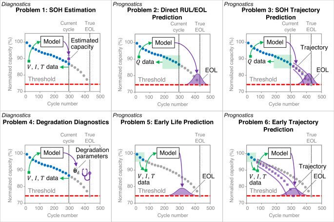
Here, V, I, T, and Q denote voltage, current, temperature, and capacity, respectively, and ({hat{{{{boldsymbol{theta }}}}}}_{{{{rm{d}}}}}) denotes an estimated vector of three degradation parameters defined to quantify three degradation modes.

Full size image

Traditional ML vs. deep learning

Over the past decade, hundreds, if not thousands, of data-driven approaches have been created for battery health diagnostics and prognostics. These existing approaches can be broadly categorized as traditional ML and deep learning. Figure 5 illustrates the key difference between these two categories. Traditional ML requires manually defining and extracting hand-crafted features. ML models are then built to approximate the often highly nonlinear relationship between these input features and the output (or target). Examples of traditional ML algorithms for building these models include regularized linear regressions (e.g., ridge regression, lasso, and elastic net), support vector machines, RVMs, Gaussian process regression (GPR) or kriging, random forests, Bayesian linear regression, gradient boosting machines (e.g., XGBoost and light gradient-boosting machines), k-nearest neighbors, and shallow neural networks.

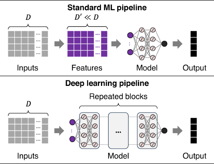
Here, a typical traditional ML pipeline requires engineers to manually identify (D{prime}) features from a D-dimensional raw input, also known as feature extraction. In contrast, a typical deep learning pipeline does not need manual feature extraction and can automatically learn features with predictive power from data.

Full size image

An input to a traditional ML model can be formulated from voltage and current measurements during a partial charge cycle. This input can be (1) a vector of features extracted from voltage vs. time (V vs. t) and current vs. time (I vs. t) curves^13,14,72, (2) a vector of features extracted from an incremental capacity vs. voltage (dQ/dV vs. V) curve^73,74, (3) a vector of features extracted from a differential voltage vs. capacity (dV/dQ vs. Q) curve⁷⁵, or (4) any combination of these three vectors⁷⁶. The output can be capacity or resistance for SOH estimation or EOL/RUL for health prognostics. The performance of ML models highly depends on the collective predictive power of these manually extracted features. Additionally, the same set of features that works well on a specific battery chemistry and application often does not transfer to a different chemistry or application. Thus, when dealing with a new chemistry or application, one has to repeat the tedious and time-consuming process of manual feature extraction.

Unlike traditional ML, deep learning can automatically learn high-level abstract features of predictive power from large volumes of data. An obvious benefit is that manual feature extraction is no longer needed and is replaced by “feature learning”. However, deep learning approaches have two well-known limitations. First, deep neural network models are more prone to overfitting data than shallower neural network models, especially when a training dataset is small (e.g., a few tens to hundreds of training samples). Given the time- and resource-demanding aging tests, most battery health diagnostics and prognostics applications reside in the small data regime⁷⁷. Aging data available for model training are even more limited in an early research and development stage where lifetime prognostics may be applied to accelerate materials design⁷⁸ or charging protocol optimization⁷⁹. As a result, a deep learning model built for battery diagnostics/prognostics may produce high accuracy on the dataset this model was trained on but may generalize poorly to “unseen” test samples that could fall outside of the training data distribution. These out-of-training-distribution test samples are often called out-of-distribution (OOD) samples. A solution to the conflict between what is needed (i.e., big data) and what is available (i.e., small data) is quantifying the predictive uncertainty through probabilistic deep learning³⁴. The uncertainty estimate could serve as a proxy for model confidence, i.e., how confident this model is when making a prediction. The ability to convey model confidence is crucial for safety-critical battery applications, where SOH/lifetime predictions with large errors and no warnings are simply unacceptable. Second, deep learning models are inherently “black-box” models whose predictions do not come naturally with an interpretation. A direct consequence is that it is almost impossible to understand why a deep learning model predicts a certain outcome and whether this prediction is reasonable and complies with physics or domain knowledge. Although efforts have been made to achieve varying degrees of interpretability mostly through post-processing⁸⁰, deep learning models are still harder to interpret than simpler traditional ML models, some of which are inherently interpretable⁷⁷.

Traditional ML models are likely to perform better on small training sets (N < 1000) than deep learning models. It is not surprising to see battery aging datasets with less than 100 cells tested to their EOL⁴⁸. In such cases, a training set may consist of only N < 100 input-output pairs. Simple ML methods such as the elastic net, a regularized linear regression method, random forests (RFs), and Bayesian linear regression are probably the best choices^27,77,81. Deep learning approaches, such as deep neural networks, are well-suited for applications where (1) it is reasonably feasible to run large-scale aging test campaigns to generate large training sets (N ≫ 1000) and (2) model interpretability is not a primary concern.

Publicly available battery aging datasets

Publicly available battery aging datasets have enabled a majority of the research in the battery diagnostics and prognostics field. The University of Maryland’s Center for Advanced Life Cycle Engineering (CALCE)^82,83,84 and the National Aeronautics and Space Administration’s (NASA)^85,86 were among the first organizations to publish publicly available battery aging datasets with greater than 20 cells. The initial work by the team at NASA focused on using an unscented Kalman filter to estimate internal battery states, namely max discharge capacity and internal resistance, and electrochemical model parameters over the course of the cells’ lifetime⁸⁶. Notably, the battery cells in the NASA dataset were subjected to randomized discharge current loads, making the dataset more similar to real-world battery operation and making it more challenging to estimate the cells’ SOH and predict their RUL. The researchers at CALCE first demonstrated RUL prediction on their dataset by using an empirical battery degradation model where the parameters are initialized using Dempster-Shafer theory and updated online using recursive Bayesian filtering⁸². The model was shown to provide accurate non-parametric predictions of battery RUL by evaluating the many Bayesian-filtered model parameters.

While the battery aging datasets from NASA and CALCE were undoubtedly influential for their time, the trend as of late has been to test more batteries under more operating conditions so that modern machine and deep learning models can be applied⁴⁸. A more recent battery aging dataset from Stanford, MIT, and Toyota Research Institute was used to study the problem of early lifetime prediction (see the section “Early life and trajectory prediction”)²⁷. The researchers then used the early lifetime prediction model in a close-loop optimization algorithm to speed up the process of experimentally searching for a fast charging protocol that maximized a cell’s cycle life⁷⁹. Similar work by a team of researchers at Argonne National Laboratory used a diverse dataset composed of 300 pouch cells with six unique battery cathode chemistries to study the role of battery chemistry and feature selection in early life prediction⁸⁷. Other large datasets include the one from Sandia National Laboratory that was used to study commercial 18650-size NMC-, NCA-, and LFP-Gr cells under different operating conditions⁸⁸ and the dataset from Oxford⁸⁹ used to study the path-dependency of battery degradation.

A relatively new dataset from the collaborators at Stanford, MIT, the Toyota Research Institute, and the SLAC National Accelerator Laboratory consists of more than 360 21,700-size automotive cells taken from a newly purchased 2019 Tesla Model 3 to study aging under a wide range of cycling conditions⁵⁵. Another large dataset made available this year is the dataset from a research collaboration between Iowa State University (ISU) and Iowa Lakes Community College that contains 251 Li-ion cells cycled under 63 unique cycling conditions²⁶. Both large aging datasets were curated specifically to study ML-based approaches to battery health prognostics and the role of feature generation and engineering in battery lifetime prediction.

Recently, there has been a push to demonstrate battery diagnostic and prognostic algorithms that work on modules and packs operating in the field. One approach to do this is to replicate real-world operating conditions in cell-level laboratory aging experiments. Pozzato et al.⁹⁰ cycled NMC/Gr+Si 21700 format cylindrical cells using a typical EV discharge profile while periodically characterizing cell health with RPTs. Similarly, Moy et al.⁹¹ cycled 31 cells using synthetically generated autonomous EV discharge profiles based on real-world driving telemetry data. While the datasets are still useful for studying battery degradation under more realistic conditions, they are still synthetic in nature and conducted on cells, making it difficult to understand how the study results translate to real-world packs and modules.

Research into module and pack based battery aging is becoming more prevalent. She et al.⁹² examined telemetry data from electric city buses operated in Beijing, China, finding that incremental capacity features extracted from the voltage readings during constant current charging were predictive of battery health, but changed drastically with the changing seasons (summer, fall, winter, spring) in the city. Similarly, Pozzato et al.³¹ looked at real-world EV data from an Audi E-tron. The team found that DC resistance measured during braking and acceleration along with charging impedance were good predictors of battery SOH. But unfortunately, neither of the aforementioned datasets were made publicly available, and to the best of our knowledge, no other publicly available battery module/pack aging datasets exist.

Publicly available battery aging datasets will continue to play a large role in furthering research in the area of battery diagnostics and prognostics by enabling those without access to battery testers to study battery aging and diagnostic and prognostic modeling. Websites like Battery Archive are important for sharing and disseminating battery aging data to a wider audience. Additionally, industry-academia collaboration will be key for gathering and disseminating real-world battery module/pack aging data. Access to real-world battery pack aging data will be crucial for studying and developing diagnostic and prognostic algorithms that can work beyond the lab. The next big leap in the battery health diagnostics and prognostics research community will be to understand how models built using lab data perform in the field.

Probabilistic ML techniques and their applications to battery health diagnostics and prognostics

This section introduces a handful of probabilistic ML/deep learning methods for building reliable probabilistic ML pipelines for battery state estimation (see an illustrative flowchart in Fig. 6 in the context of capacity estimation). Following the introduction of each probabilistic ML method, we review the state-of-the-art in applying this method to solve the first three problems (Problems 1–3) on battery diagnostics/prognostics shown in Fig. 4, i.e., SOH estimation, capacity forecasting, and RUL prediction. The other three problems (Problems 4–6) are emerging and will be discussed in “RVM applications to battery diagnostics and prognostics SOH estimation”.

Among the probabilistic ML algorithms listed here, “GPR” stands for Gaussian process regression (the section “Gaussian process regression”); “RVM” stands for relevance vector machine (the section “Relevance vector machine”); “sampling stands for sampling methods (the section “Sampling methods”); “BNN” stands for Bayesian neural network (the section “Bayesian neural network”); “MC dropout” stands for Monte Carlo dropout (the section “Bayesian neural network”); and “NN ensemble” stands for neural network ensemble (the section “Neural network ensemble”).

Full size image

As one proceeds through this section, one will notice that it goes beyond merely addressing the theoretical and battery application aspects of each probabilistic ML technique covered. It also includes specific algorithm examples (e.g., Figs. 7–12) and offers a tutorial-style description of the algorithmic procedures. Our aim is to present easily digestible materials, particularly for newcomers in this field, such as fresh Ph.D. students eager to grasp the fundamentals of probabilistic battery diagnostics and prognostics. We also note that there exists a broader spectrum of probabilistic ML methods beyond those discussed in this paper (e.g., see Nemani et al.³⁴); we aim in this paper to highlight a select few that have been most prominently used in, and generally applicable, to the type of problems encountered in battery diagnostics and prognostics.

Here, the 95% prediction interval (denoted as “PI” in the legend) represented by the shaded area is computed as μ_* ± 2σ_*.

Full size image

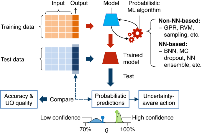
Before we introduce the probabilistic ML methods, it is meaningful to walk through some key steps when applying probabilistic ML to battery state estimation. As a representative example, Fig. 6 provides a graphical overview of these key steps for capacity estimation. Similar steps can be expected when solving other problems on battery diagnostics and prognostics.

• This pipeline starts with defining an ML model’s input and output. For example, when dealing with capacity estimation by traditional ML models, the input could consist of predictive features extracted from the voltage (V), current (I), and temperature (T) measurements during a partial charge cycle, and the output would be the full capacity (Q) of the cell at that cycle.

• The next step is defining a training and test dataset. An important consideration is that the test dataset should include a decent number (e.g., ≥30%) of OOD samples to evaluate the generalization performance of a trained ML model. Furthermore, one should avoid randomly assigning samples from the same cell to both training and test datasets. In most cases, all samples from one cell should be exclusively assigned to a training or test dataset. Again, this treatment ensures that the test dataset serves the purpose of evaluating how well a trained ML model generalizes to samples outside of the dataset the model has been trained on.

• The third step is selecting a probabilistic ML algorithm. This section covers three non-neural-network-based algorithms, GPR (the section “Gaussian process regression”), RVM (the section “Relevance vector machine”), and sampling methods (the section “Sampling methods”), and two neural-network-based algorithms, BNN (the section “Bayesian neural network”) and neural network ensemble (the section “Neural network ensemble”). Selecting a probabilistic ML algorithm requires assessing several criteria to ensure the algorithm’s suitability for a specific use case. Several key criteria are listed as follows (see Nemani et al.³⁴ for further details): (1) prediction accuracy (e.g., evaluated by comparing mean predictions with ground truth on a validation dataset spit out of a training dataset), (2) quality of uncertainty quantification (i.e., the algorithm’s ability to produce accurate uncertainty estimates), (3) computational efficiency (an important factor in applications where real-time or near-real-time diagnostics/prognostics may be required), (4) scalability (i.e., the algorithm’s ability to train models based on large volumes of datasets, i.e., in the big data regime), and (5) robustness (i.e., the algorithm’s ability to maintain performance in the presence of outliers, high noise, and adversarial variations in the input data). These criteria may become conflicting objectives that need to be weighed based on the needs and wants of a specific diagnostic/prognostic use case. It is often desirable to experiment with a suite of algorithms and choose one (standalone) or multiple (hybrid) algorithms for a specific use case.

• After selecting the algorithm, one feeds the training data, some observed input-output pairs, into the algorithm. This algorithm then generates a mathematical model that infers something about the underlying process that generated the training data. Using the trained model, one can make probabilistic capacity estimations for cells or their cycle numbers the model has not seen before. Each capacity estimate can be expressed as a probability distribution of a certain type (e.g., Gaussian, log-normal, or exponential) or an empirical probability distribution.

• If one has access to the ground truth for the test data, one can compare the capacity estimates with the observations to derive prediction accuracy metrics, such as the root-mean-square error (RMSE) and mean absolute percentage error, and uncertainty quantification quality metrics, such as the expected calibration error, Area Under the Sparsification Error curve (AUSE), and negative log-likelihood (NLL).

Gaussian process regression methodology

Gaussian process regression (GPR), also known as kriging, is a principled, probabilistic method for learning an unknown function f from a given set of training data comprising N input vectors, ({left{{{{{bf{x}}}}}_{i}right}}_{i = 1,ldots ,N}), and N targets, ({left{{y}_{i}right}}_{i = 1,ldots ,N}). Here, ({{{{bf{x}}}}}_{i}in {{mathbb{R}}}^{D}) is the D-dimensional input feature vector of the i-th training sample, and ({y}_{i}in {mathbb{R}}) is the corresponding one-dimensional output, i.e., a noise-free or noisy observation of f at x_i. The regression model learned by GPR is non-parametric because this model does not have a predefined functional form. It is common to assume the so-called Gaussian observation model where each observation y_i is an addition of the true function value f(x_i) and a zero-mean Gaussian noise ε_n:

where ({varepsilon }_{i} sim {{{mathcal{N}}}}(0,{sigma }_{varepsilon }^{2})). GPR starts by placing a Gaussian process prior on the unknown function f, i.e., (f({{{bf{x}}}}) sim {{{mathcal{GP}}}}(m({{{bf{x}}}}),k({{{bf{x}}}},{{{{bf{x}}}}}^{{prime} }))), where m(⋅) is the mean function and k(⋅,⋅) is the kernel, also known as the covariance function evaluated at x and ({{{{bf{x}}}}}^{{prime} })⁹³. For example, if we assemble the N function values into a vector, ({{{bf{f}}}}={[f({{{{bf{x}}}}}_{1}),ldots ,f({{{{bf{x}}}}}_{N})]}^{{{{rm{T}}}}}), this vector follows a multivariate (N-dimensional) Gaussian distribution:

where ({{{bf{X}}}}={[{{{{bf{x}}}}}_{1},ldots ,{{{{bf{x}}}}}_{N}]}^{{{{rm{T}}}}}in {{mathbb{R}}}^{Ntimes D}) is a matrix assembly of the N training input points, m(X) is a vector of the mean values at these input points, and ({{{{bf{K}}}}}_{{{{bf{X}}}},{{{bf{X}}}}}in {{mathbb{R}}}^{Ntimes N}) is a covariance matrix that takes the following form:

Nonlinearity in the model arises from the kernel k(⋅,⋅), which models the covariance between function values at two different input vectors. In practice, we can choose a kernel from many candidates. For example, the probably most popular kernel is the squared exponential kernel, also known as the radial basis function (RBF) and the Gaussian kernel. The squared exponential kernel can be expressed as

where σ_f is the signal amplitude, ∥⋅∥ is the L2 norm or the Euclidean norm, the square of which (({sigma }_{f}^{2})) defines the signal variance, and l is the length scale. The signal variance (({sigma }_{f}^{2})) sets the upper limit of the variance and covariance for the Gaussian process prior (see the covariance matrix in Eq. (2); the length scale l determines how smooth the approximate function appears (the smaller the length scale, the more rapidly the function changes). These two kernel parameters are two hyperparameters of the GPR model, which, together with the noise standard deviation σ_ε, need to be optimized during GPR model training. The squared exponential kernel has been widely used as it is simple and captures a function’s stationary and isotropic (dimension-dependent) behavior. Another popular choice is the RBF kernel with automatic relevance determination (ARD)⁹⁴, which assigns N different length-scale parameters to the N dimensions rather than using the same parameter as is done by the standard RBF kernel. The resulting RBF-ARD kernel can capture dimension-dependent patterns in the covariance structure.

For notational convenience, we denote the collection of training input-output pairs as a training set, ({{{mathcal{D}}}}=left{left({{{{bf{x}}}}}_{1},{y}_{1}right),ldots ,left({{{{bf{x}}}}}_{N},{y}_{N}right)right}), and write the N noisy observations as a vector, ({{{bf{y}}}}={[{y}_{1},ldots ,{y}_{N}]}^{{{{rm{T}}}}}in {{mathbb{R}}}^{N}). For a new, unseen input point x_*, the predictive distribution of the corresponding observation y_* can be derived based on the conditional distribution of a multivariate Gaussian as the following:

and

where (k({{{bf{X}}}},{{{{bf{x}}}}}_{* })={[k({{{{bf{x}}}}}_{1},{{{{bf{x}}}}}_{* }),ldots ,k({{{{bf{x}}}}}_{N},{{{{bf{x}}}}}_{* })]}^{{{{rm{T}}}}}), denoting a vector of N cross covariances between X and x_*.

GPR is a probabilistic ML method most well-known for its distance-aware uncertainty quantification capability. This capability is illustrated in Fig. 7, where a simple sine function is adopted to generate synthetic data after adding zero-mean Gaussian noise. Two observations can be made from this figure. First, high epistemic uncertainty due to a lack of data is associated with test points far from the eight training points. The GPR model seems to produce predictive uncertainty estimates that properly capture the high epistemic uncertainty at these OOD test points. Second, as a test point deviates from the training data distribution (e.g., when x starts to become larger than 4), the predictive uncertainty first increases due to the distance-aware property of GPR and then saturates to a maximum constant (i.e., ({sigma }_{* }^{2},approx, {sigma }_{f}^{2}+{sigma }_{varepsilon }^{2})). The above briefly overviews the math behind GPR and its uncertainty quantification capability. Our recent tutorial on uncertainty quantification of ML models³⁴ provides a more detailed explanation of GPR.

Figure 8 shows how GPR operates to forecast the capacity of future cycles probabilistically at a specific charge/discharge cycle. We first train a GPR model based on the available capacity data (blue points). This GPR model uses an empirical capacity fade model as the prior mean function to capture the known fade trend. The model training optimizes the GPR model’s hyperparameters by maximizing the likelihood of observing the capacity data. Intuitively, we fit a GPR regression model to available capacity data and use this model to make predictions for future cycles without capacity data. Because GPR is a probabilistic ML technique, the predictions are in the form of a mean curve, the solid line, and a 95% prediction interval, the dashed lines. So, in the next step, we forecast capacity beyond the current cycle using the trained GPR model, making predictions outside our data distribution. We then estimate the mean EOL when the mean prediction curve down-crosses a predefined capacity threshold or EOL limit. The black square is the mean prediction. We can imagine having a prediction interval around this mean, representing the uncertainty of our EOL prediction. We are often interested in knowing the RUL, i.e., the number of remaining cycles till the EOL limit. Our RUL estimate can be obtained by simply subtracting the current cycle number from the predicted EOL. Since this device was cycled to its EOL, we have the entire capacity trajectory and true EOL. We can compare the prediction and truth to know how well our GPR model does.

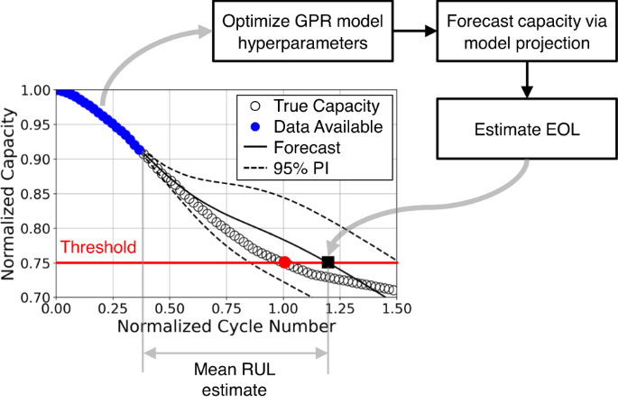
Here, the GPR model is fit to available data and extrpolated to forecast capacity and EOL.

Full size image

Now imagine we repeat the prediction steps in Fig. 8 at every cycle, as the battery is used in the field. Figure 9 shows how the prediction evolves from an early-life cycle to a late-life cycle. This figure panel shows six snapshots of probabilistic capacity forecasting by GPR at six different cycles. As we move along the cycle axis, we have more and more capacity data to train a GPR model and our prediction horizon till the EOL becomes shorter and shorter. As a result, the EOL and RUL predictions become more and more accurate. These predictions converge to the ground truth at around halfway through the lifetime. Also, We can see the prediction interval for the EOL, in general, gets narrower with time, indicating reduced predictive uncertainty, which is also what we expect to see.

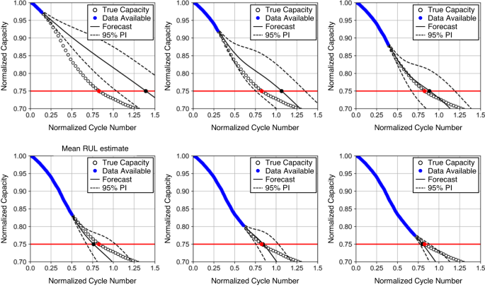
Here, the GPR model is fit to available date and extrapolated to EOL. The various lengths of data available change the projected trajectory.

Full size image

SOH estimation

Two notable efforts applying GPR to SOH estimation were made almost simultaneously^72,95. Both studies extracted features from the raw voltage vs. time (V vs. t) curve acquired from a charge cycle. Richardson et al.⁷² used the time differences between several equispaced voltage values and their minimum as the input features to a GPR model. These time differences were computed based on a segment of a full charge curve (after smoothing) within its constant-current (CC) portion. Yang et al.⁹⁵ took a different feature engineering path by extracting time and slop features from a full charge curve consisting of both the CC and constant-voltage portions. It is noted that earlier studies on SOH estimation investigated similar features extracted from a charge curve starting at a partially discharged state^13,96. Both studies^72,95 evaluated their algorithms on a battery aging dataset from the NASA Ames Prognostics Center of Excellence Data Set Repository (e.g., the Randomized Battery Usage dataset⁸⁶ used in ref. ⁷².

These two early applications of GPR to SOH estimation reported two unique properties of GPR: nonparametric regression, making the regression model self-adaptable to data complexity, and uncertainty estimation under a Bayesian framework and with distance awareness, enabling principled quantification of predictive uncertainty and reliable detection of OOD samples. Additionally, GPR is known for its minimal overfitting risk due to using a Bayesian probabilistic framework. These desirable properties may have driven many later studies that investigated the applicability of GPR to SOH estimation when only partial charge curves are available. Two examples of such investigations examined features extracted from the incremental capacity vs. voltage curve during partial charge⁷³ and features extracted from the capacity vs. voltage curve during partial charge⁹⁷. As discussed next, GPR can extrapolate reasonably well when a prior mean function is properly defined. However, GPR only operates well on small datasets and has limited scalability to bigger datasets³⁴.

SOH forecasting and RUL prediction

The first application of GPR in the battery diagnostics and prognostics literature was SOH forecasting, not SOH estimation. It was reported in a comparative study on resistance and capacity forecasting led by a group of researchers at NASA’s Ames Research Center⁹⁸. This study compared two regression techniques, polynomial regression and GPR, and one state estimation technique, particle filtering, in forecasting resistance and capacity. This comparative study was an extended version of the probably first-ever publication on battery diagnostics/prognostics, led by the same group of researchers¹¹, which used a combination of RVM and particle filtering for capacity forecasting. SOH forecasting using GPR has an ~10-year longer history than SOH estimation using GPR. After the first application of GPR to SOH forecasting in the late 2000s, two notable studies attempted to improve the extrapolation performance of GPR, essential to long-term SOH forecasting, by using explicit prior mean functions^99,100. Note that the default option for the prior mean function is either zero or a non-zero constant⁹³. An empirical capacity fade model could be used as an explicit mean function, allowing the GPR model to capture the trend of degradation encoded in the capacity fade model^100,101.

All the above studies on SOH forecasting assume that use conditions (e.g., charge and discharge C-rates and temperature) are time-invariant. This assumption may not hold in many real-world applications. A more realistic scenario is that these use conditions vary randomly over time but approximately follow a duty cycle pattern. As a follow-up to their earlier study on SOH forecasting¹⁰², Richardson et al. defined a capacity transition model to predict the capacity change during each usage period following a load pattern. A GPR model was built to approximate the relationship between features extracted from a load pattern (input) and the capacity change within this usage period (output). The outcome was the ability to forecast capacity probabilistically under time-varying use conditions. Two more recent studies also examined capacity forecasting under time-varying use conditions, specifically in cases where future charge and discharge C-rates vary significantly with cycle^103,104. Similar to the study by Richardson et al.¹⁰², these two more recent studies also consider future use conditions when designing the input to an ML model. Specifically, they used charge and discharge currents in future cycles as part of the ML model input. The difference is that these two studies additionally incorporated the current or recent cell state into the model input. The cell state was characterized by either (1) a combination of features from electrochemical impedance spectroscopy (EIS) measurements in the current cycle and those from voltage and current measurements in the current and some past cycles¹⁰³ or (2) only features from historical voltage and current measurements¹⁰⁴. GPR was not used as the ML algorithm in either study. Instead, an ensemble of XGBoost regressors was used by Jones et al.¹⁰³ to quantify forecasting uncertainty, while uncertainty quantification was not considered by Lu et al.¹⁰⁴. Overall, it is interesting to see both studies focused on features with physically meaningful connections to future degradation when designing the ML model input. In fact, formulating a meaningful forecasting problem and designing highly predictive input features should be the centerpiece of almost any data-driven SOH forecasting effort.

Finally, it is worth noting that multiple probabilistic ML models can be combined to form a hybrid model for SOH forecasting or RUL prediction. In what follows, we briefly discuss three examples of hybrid modeling involving GPR.

• The first example is the delta learning approach employed by Thelen et al. in their study on battery RUL prediction¹⁰¹. The basic idea of this approach is correcting initial RUL predictions by a GPR capacity forecasting model with a data-driven ML model. The prior mean function of the GPR model was explicitly designed to be an empirical capacity fade model. The approach was demonstrated on three open-source datasets, a simulated dataset, and one proprietary dataset. Initial RUL predictions by GPR capacity forecasting models were considerably under-confident as compared to the GPR delta learning approach with a GPR capacity forecasting model (predictor) and a GPR RUL error correction model (corrector), which was well calibrated on the original dataset. In contrast, the random forest delta learning approach using a probabilistic random forest model as the corrector was over-confident on the original dataset, but exhibited better calibration than the GPR delta learning approach on the simulated OOD dataset.

• Another example is the use of a co-kriging model to forecast capacity degradation by combining two data sources: (1) a high-fidelity source consisting of the capacity measurements from the test cell (whose capacity trajectory beyond the current cycle needs to be predicted) up to the current cycle and (2) a low-fidelity source comprising capacity measurements from other cells of the same or a similar design¹⁰⁵. Similar to the delta learning approach studied by Thelen et al.¹⁰¹, this second study attempted to build a corrective GPR model to compensate for the deviation of an initial GPR model built based on low-fidelity data to depict an “average” degradation trajectory.

• The third example is an effort to modify vanilla GPR models by incorporating electrochemical and empirical knowledge of capacity degradation (i.e., the dependencies of capacity degradation on two cycling condition variables, named temperature and depth of discharge)¹⁰⁶. These two dependencies were captured through the Arrhenius law (temperature) and a polynomial equation (depth of discharge), respectively, and encoded as a compositional covariance function (or kernel) within GPR. Unlike the first two examples, which are purely data-driven, this third example attempted to integrate some physics of degradation into the GPR formulation, which can be treated as a physics-informed probabilistic ML approach.

Relevance vector machine methodology

Suppose we have access to a set of training samples, each sample consisting of an input–output pair, (x_i, y_i), i = 1, ⋯ , N, where ({{{{bf{x}}}}}_{i}in {{mathbb{R}}}^{D}) is the D-dimensional input features of the i-th training sample, ({y}_{i}in {mathbb{R}}) is the corresponding output (also known as the target or the observation of the state of interest), and N is the number of samples. We are interested in learning a one-to-one mapping from the input (feature) space to the output (state) space. Similar to GPR, RVM also assumes that the observations are samples from a Gaussian observation model. Unlike GPR, which does not assume any functional form of this mapping, RVM approximates this mapping as a parametric, linear kernel regression function¹⁰⁷. This regression function takes the following form:

where x is an input feature vector whose target may be unknown and needs to be inferred, K(x, x_i) is a kernel function comparing the test input x with each training input x_i, ω_i is the kernel weight measuring the importance (or relevance) of the ith training sample, ω₀ is a bias term, and ε is a zero-mean Gaussian noise, i.e., (varepsilon sim {{{mathcal{N}}}}(0,{sigma }_{varepsilon }^{2})). The bias term and N kernel weights form a (N + 1)-element weight vector, written as ({{{boldsymbol{omega }}}}={[{omega }_{0},{omega }_{1},ldots ,{omega }_{N}]}^{{{{rm{T}}}}}). If we define a design vector consisting of a constant of one and the N kernel functions, i.e., ({{{boldsymbol{phi }}}}={[K({{{bf{x}}}},{{{{bf{x}}}}}_{1}),ldots ,K({{{bf{x}}}},{{{{bf{x}}}}}_{N})]}^{{{{rm{T}}}}}), we can rewrite Eq. (7) in a convenient vector form, y(x) = ω^Tϕ + ε. The original RVM formulation follows a hierarchical Bayesian procedure by assuming the (N + 1) weights follow a zero-mean Gaussian prior, whose inverted variances, denoted as ({left{{alpha }_{i}right}}_{i ,=, 0,cdots ,N}), and the inverted noise variance, ({sigma }_{varepsilon }^{-2}), all follow Gamma distributions (hyperpriors).

Training the model in Eq. (7) using sparse Bayesian learning estimates the posterior of the weight vector ω and noise variance ({sigma }_{varepsilon }^{2}) via iterative optimization¹⁰⁷. In practice, the posterior for most weights becomes highly peaked at zero, effectively “pruning” the corresponding kernel functions from the trained model. The remaining training samples with non-zero weights are known as relevance vectors, typically accounting for a very small portion of the training set (e.g., 5−20%). This unique attribute of sparsity makes the RVM attractive both in terms of generalization performance and test-time efficiency.

Figure 10 illustrates battery capacity estimation by a trained RVM model based on features extracted from voltage and current measurements during partial charge¹³. This SOH estimator possesses two desirable attributes: (1) statistical estimation, i.e., instead of providing a mere point estimate for the SOH parameter, this estimator generates a probability distribution as the parameter estimate; (2) sparsity, i.e., the estimator selectively utilizes only a small subset of feature vectors from the training dataset, known as relevance vectors, for real-time health inference (see, for example, the extreme posterior peakness at zero for ω₂ and ω_N). These two attributes offer several advantages for online health inference: (1) statistical estimation enables concurrent estimation of the parameter while quantifying the associated uncertainty, and (2) sparsity enhances the computational efficiency of online inference.

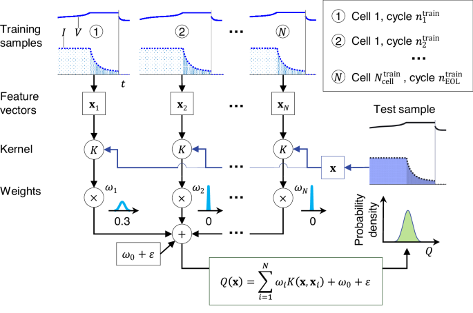
Example ML pipeline for capacity estimation using RVM trained on voltage-time and current-time data during cell charging. Figure adapted from Fig. 2 in Hu et al.¹³

Full size image

SOH estimation

As shown in Fig. 10, RVM can be applied to estimate battery capacity from features extracted from readily available voltage and current measurements. Such applications were first attempted in two studies, one focusing on implantable-grade LCO cells¹³ and the other focusing on NMC cells¹⁰⁸. In the former study¹³, five characteristic features, some correlated strongly with capacity, were extracted from a test cell’s voltage vs. time and current vs. time curves at a specific charge cycle that started at a partially discharged state. These features were then fed as input (e.g., x in Fig. 10) into a trained RVM regression model that produced as output a Gaussian-distributed capacity estimate (e.g., Q in Fig. 10). The sparsity property of RVM made this regression model much smaller than a full-scale model. For example, each cross-validation trial used only <4% of training samples as the relevance vectors to build the final regression model, improving the computational efficiency and generalization of online capacity estimation.

In the later study¹⁰⁸, a feature of predictive power was found to be the sample entropy of a short voltage sequence (time series) measured during a hybrid pulse power characterization test. This feature was concatenated with temperature to form the input vector to an RVM regression model, which outputs a Gaussian-distributed capacity estimate. It is interesting to see the inclusion of use condition parameters (e.g., temperature as reported in Hu et al.¹⁰⁸) in the input of a data-driven ML model. Such a treatment builds condition awareness into the ML model, making it applicable under varying use conditions. Similar approaches have been taken in studies on capacity forecasting, as discussed in the section “GPR applications to battery diagnostics and prognostics”.

It is also widely accepted that a “one-ML-method-fits-all” approach does not work in battery diagnostics and prognostics. In some applications, one ML method may perform better than another regarding prediction accuracy. But, in other applications, accuracy comparisons between these two methods may look very different. Some limited efforts have been made to benchmark different ML methods for SOH estimation. An example is a comparative study on four data-driven ML methods, namely linear regression, support vector machine, RVM, and GPR, using features extracted from capacity vs. voltage curves during discharge¹⁰⁹. These features included the standard deviations of the discharge capacity (Q) and cycle-to-cycle discharge capacity difference (ΔQ), calculated, respectively, from a measured sample of the discharge capacity vs. voltage curve at the current cycle (Q(V)) and a measured sample of the discharge capacity difference (between the current cycle and a fixed early cycle) vs. voltage curve (ΔQ(V)).

Like most other studies on battery diagnostics and prognostics, the above comparison exclusively focused on prediction accuracy by looking at error metrics such as RMSE and maximum absolute error. Few research or benchmarking efforts were made to study the quality of uncertainty quantification, i.e., how well an estimate of a model’s predictive uncertainty (known) on a test sample reflects the model’s prediction error (unknown) on this sample³⁴. Additionally, we see that most studies worked with small datasets from limited numbers (mostly <100) of cells. In the small data regime, examining predictive uncertainty is even more important than in the big data regime, simply because (1) small training datasets possess limited representativeness of real-world scenarios, and (2) ML models may generalize poorly to OOD data. Although these existing studies reported high accuracy on small, carefully crafted test datasets mostly acquired from laboratory testing, these accuracy numbers are unlikely to generalize to real-world applications where we would expect wider ranges of and more complex use conditions, higher cell-to-cell variability, and larger measurement noise.

SOH forecasting and RUL prediction

The first application of RVM to battery prognostics was pioneered by a group of researchers at NASA’s Ames Research Center¹¹. The same group of researchers also led the first application of GPR to battery prognostics⁹⁸, as discussed in the section “RVM applications to battery diagnostics and prognostics SOH estimation”. The role RVM served was identifying mean regression curves on a charge transfer resistance vs. time dataset and electrolyte resistance vs. time dataset, both acquired from EIS. Each mean regression curve was then fitted to a simple two-parameter exponential model to obtain an estimate of the two model parameters. This estimate was treated as an initial (t = 0) estimate of the exponential model parameters in a discrete-time state-space model, solved using particle filters for capacity forecasting and RUL prediction. RUL prediction results were shown as an empirical probability distribution that became narrower and more centered at the true RUL as the cycle number where the prediction was made increased. Such plots later became a standard way to visualize results by probabilistic RUL prediction methods^{82,110,111,112}.

Two later, more direct applications of RVM to battery prognostics were explored with the formulation of two vastly different approaches^12,113. Wang et al. performed RVM regression on the capacity vs. cycle number data available to a test cell whose future capacity and RUL were unknown and then fitted a three-parameter variant of the well-known double exponential capacity fade model⁸² to only the capacity (Q) and cycle number (t) data of the relevance vectors¹². Capacity forecasting and RUL prediction were achieved by extrapolating the fitted capacity fade model to a predefined EOL limit. It is important to note that, similar to the first application⁹⁸, the RVM regression model, fitted to an SOH vs. cycle number dataset, was not directly used for capacity forecasting. More specifically, the forecasting was not done by extrapolating the RVM regression model, unlike the capacity forecasting studies using GPR models with empirical fade models as the “built-in” prior mean functions, as discussed in “RVM applications to battery diagnostics and prognostics SOH estimation”. Li et al. took a different approach by formulating capacity forecasting as a time series prediction problem¹¹³. RVM was employed to map the current and several past cycles’ capacity observations to the next cycle’s capacity observation, enabling one-step-ahead prediction. Capacity observations at cycles beyond the next cycle were predicted via iterative one-step-ahead prediction (i.e., marching over time). Again, capacity forecasting was not achieved by extrapolating an RVM regression model fitted to capacity vs. cycle number data. It suggests that simply extrapolating a data-driven regression model without consideration of the capacity fade trend may not yield reliable capacity forecasting, especially for long-term forecasting.

Bayesian neural network methodology

A neural network f_NN makes a prediction for an output variable at an input feature: (hat{y}={f}_{{{{rm{NN}}}}}({{{bf{x}}}};{{{boldsymbol{theta }}}})), where θ denotes all tunable parameters of the neural network (e.g., the neural network weight and bias terms). Given training samples (x_i, y_i), i = 1, ⋯ , N, the neural network training process seeks to set θ = θ^* that minimizes a loss function, commonly the mean squared error:

This optimization problem is typically solved via gradient-based algorithms such as stochastic gradient descent^114,115 or Adam¹¹⁶. The resulting θ^* is single-valued, and subsequent new prediction using this trained neural network would also be single-valued as well: ({hat{y}}_{{{{rm{new}}}}}={f}_{{{{rm{NN}}}}}({{{{bf{x}}}}}_{{{{rm{new}}}}};{{{{boldsymbol{theta }}}}}^{* })).

In order to capture the uncertainty in determining θ, one can solve for θ in a probabilistic manner following the Bayesian framework^117,118,119, and seek the entire distribution of plausible θ values instead of a single-valued “best fit”. Such an approach entails constructing a Bayesian neural network (BNN). In a BNN, θ is treated as a random variable with an associated probability density function (PDF) representing its uncertainty. When training data become available, the PDF of θ is updated following Bayes’ rule:

where p(θ∣x, y) is the posterior PDF (updated uncertainty given training data), p(θ) is the prior PDF (initial uncertainty before seeing training data), p(y∣x, θ) is the likelihood PDF, and p(y∣x) is the marginal likelihood or model evidence that is constant with respect to θ. Solving the Bayesian inference problem constitutes computing or characterizing the posterior p(θ∣x, y). Once the posterior becomes available, its uncertainty can be propagated to predictions by first drawing posterior samples θ⁽ⁱ⁾ ~ p(θ∣x, y) and then evaluating the neural network ({hat{y}}_{{{{rm{new}}}}}^{(i)}={f}_{{{{rm{NN}}}}}({{{{bf{x}}}}}_{{{{rm{new}}}}};{{{{boldsymbol{theta }}}}}^{(i)})) for each sample. The set of neural network predictions represent the posterior-pushforward distribution that is solely due to the epistemic uncertainty in the neural network parameters. In contrast, the posterior predictive distribution would additionally include the aleatory uncertainty from the output observation noise, often portrayed by samples in the form ({y}_{{{{rm{new}}}}}^{(i)}={f}_{{{{rm{NN}}}}}({{{{bf{x}}}}}_{{{{rm{new}}}}};{{{{boldsymbol{theta }}}}}^{(i)})+{epsilon }^{(i)}). Hence, a distribution of predicted values will be generated to reflect the residual uncertainty in the neural network model parameters.

Solving for the posterior is highly challenging for BNNs due to the high dimensionality of θ (often thousands to millions in neural networks). Markov chain Monte Carlo^{120,121,122,123}, which are classical Bayesian inference algorithms designed to generate samples from the exact posterior, do not scale well to such high dimensions in practice. The exploration-efficient Hamiltonian Monte Carlo (HMC)^124,125 has been used on some BNNs but usually for smaller cases with hundreds of parameters. Alternatively, variational inference (VI)^126,127 forms an optimization problem to find the best approximate posterior from a class of parameterized distributions. Let q(θ; λ) denote the approximate posterior density parameterized by λ, VI minimizes the Kullback-Leibler divergence from the true posterior to the approximate posterior:

where the second equation is simplified to the well-known evidence lower bound that no longer involves the marginal likelihood and can be approximated via Monte Carlo (MC) sampling. By sidestepping posterior sampling with an optimization problem, VI effectively trades off some posterior accuracy for scalability, making it more suitable for BNNs.

The simplest form of VI is the mean-field VI using Gaussians, where (q({{{boldsymbol{theta }}}};{{{boldsymbol{lambda }}}})=mathop{prod }nolimits_{k = 1}^{K}{q}_{k}({{{{boldsymbol{theta }}}}}_{k};{{{{boldsymbol{lambda }}}}}_{k})=mathop{prod }nolimits_{k = 1}^{K}{{{mathcal{N}}}}({{{{boldsymbol{theta }}}}}_{k};{mu }_{k},{sigma }_{k}^{2})) are set to independent (mean-field) Gaussians¹²⁸, involving the optimization of a 2K-dimensional λ. Gradient information for the VI optimization can also be obtained through back-propagation¹²⁸. However, such a mean-field approach cannot capture parameter correlations and tends to under-predict the uncertainty¹²⁶. While a natural extension is to incorporate a full-covariance instead of the independence assumption, however, tracking all entries of a dense covariance matrix would require ({{{mathcal{O}}}}({K}^{2}))-dimensional λ, rendering it often too expensive and thus rarely used for BNNs. Other advanced representations of q(θ; λ) are possible, for example, via normalizing flows¹²⁹ and transport maps¹³⁰ that parameterize the mapping from the posterior random variable θ to a standard normal reference random variable.

Stein variational gradient descent (SVGD)¹³¹ also approximates the posterior through an optimization problem but uses particles. SVGD leverages the relationship between the (functional) gradient of objective in Eq. (10) to the Stein discrepancy, the latter which can be approximated using a set of particles. The particles’ positions are then iteratively updated following the gradient-descent direction, transporting them towards the target posterior distribution p(θ∣x, y). Further enhancements such as Stein variational Newton^132,133 that makes use of second-order (Hessian) information, and projected SVGD¹³⁴ that finds low dimensional data-informed subspaces, have also been developed.

Lastly, MC dropout is a regularization technique for training deep neural networks¹³⁵ but has been shown to approximate the posterior predictive distribution under a specific Bayesian setup¹³⁶. Adding MC dropout to an existing deterministic deep neural network training infrastructure is very easy and essentially involves generating a set of sparse neural networks by randomly setting some weight parameters to zero. However, MC dropout is not formulated to tackle the Bayesian formulation in Eq. (9), and thus is limited in handling general choices of prior p(θ) and likelihood p(x, y∣θ).

SOH estimation

The use of BNN for battery diagnostics/prognostics has been few in number and largely lacked rigorous analysis of its Bayesian uncertainty quantification. For example, Kim et al.¹³⁷ proposed a knowledge-infused BNN for on-board SOH estimation and RUL prediction of Li-ion batteries in EVs. Their approach incorporated novel domain knowledge by (a) designing impedance-related features based on discharge voltage slopes that have been observed to be correlated with degradation, and (b) introducing into an RNN a knowledge-infused block that uses an empirical double-exponential model for degradation estimation. The RNN was then turned into a BNN via a combination with MC dropout. However, the work had no mentioning of the prior and likelihood, both central for establishing the Bayesian problem formulation in Eq. (9). Elsewhere, Xu et al.¹³⁸ built BNNs to predict the SOH of retired batteries by leveraging unique data from EIS experiments. The paper provided detailed experimental setup, data acquisition, and feature extraction highlighting the use of an equivalent circuit model and ARD. However, similar to the previous work, information regarding the BNN prior and likelihood were missing. While the paper did mention the use of VI for BNN training, it failed to clarify the VI method and what variational families were employed (e.g., if using mean-field Gaussian VI).

SOH forecasting and RUL prediction

In the work of Zhu et al.¹³⁹, the authors used MC dropout to create a general RUL prediction framework, with a demonstration example of battery degradation from a laboratory setting, that also featured an active learning procedure for choosing the next sampling point using the posterior predictive variance as the acquisition function. Hong et al.¹⁴⁰ introduced a “first full end-to-end deep learning framework” for predicting Li-ion battery RUL through a dilated CNN architecture that incorporated temporal measurements of battery terminal voltage, current, and cell temperature. The paper then used an explicit ensembling procedure (see next section) as an approximation to BNN.

In contrast to the aforementioned literature, the papers^141,142 clearly specified the prior and likelihood of their Bayesian setups along with the algorithm for solving the posterior. The former employed mean-field Gaussian VI to build a Bayesian mixture neural network in the form of a hybrid of a Bayesian CNN and LSTM, for predicting the RUL in multiple battery datasets. The latter adopted HMC and VI by backpropagation¹²⁸ to construct BNNs for general RUL prediction without focusing on batteries, and demonstrated instead on an open dataset of turbofan engines.

Overall, research for SOH and RUL prediction is seeing increasing use of BNNs, recognizing the importance of uncertainty quantification in deep learning models that generally tend to be opaque and not interpretable. However, the majority of these BNN works simply cite the connection to MC dropout without mentioning the assumptions and conditions that accompany these off-the-shelf tools. This can be a dangerous practice and lead to incorrectly quantified uncertainties not justified by the data or not intended by the modeler. More careful analysis of the Bayesian results would be warranted, for example, by diagnosing how close the dropout posterior is to the true posterior p(θ∣x, y). This would require the probing (at least recognition) of posterior results (not just posterior-predictive results and not just looking at RMSE of the predictions), which currently are often from BNN literature.

Neural network ensemble methodology

Approaches that combine predictions by multiple ML models to derive a final prediction can be categorized as ensemble learning approaches. The key idea is to introduce diversity among models in the ensemble, encouraging member models to agree more when a test sample falls inside the training data distribution and disagree more when the test sample is OOD. Diversity can be created in many different ways. The sampling methods described in the section “Sampling methodologies” can generally be treated as ensemble learning approaches. For example, bagging (a.k.a. bootstrap aggregating) builds a diverse set of member models in an ensemble by creating random subsets of the original training set and using each subset to train a member model (see Fig. 12 for an illustrative example). These methods allow making probabilistic predictions using deterministic ML techniques (e.g., the elastic net [end-to-end early prediction paper] and random forest¹⁴).

A recent effort attempted to achieve diversity among neural networks by training multiple neural networks of the same architecture, each with a random (thus different) parameter initialization and a unique sequence of randomly sampled mini-batches, i.e., simply following the standard stochastic gradient descent procedure¹⁴³. The resulting ensemble captures the predictive uncertainty due to observational noise in the target (y) of an aleatory nature and insufficient training data of an epistemic nature. This recent effort specifically targeted uncertainty quantification of deep neural networks, as they produced state-of-the-art prediction accuracy on many benchmarking problems but had been found to give often over-confident predictions. These predictions, if incorrect, can quickly diminish the value of predictive modeling in safety-critical applications and substantially damage users’ trust in the ML model.

Constructing a neural network ensemble involves (1) training individual neural networks, of which each predicts a Gaussian-distributed output capturing aleatory uncertainty, and (2) aggregating the Gaussian predictions by these individual models as a Gaussian mixture to capture epistemic uncertainty. These two steps are illustrated in Fig. 11 and detailed below in the context of battery capacity estimation.

• Step 1: Training multiple neural networks with Gaussian output layers Suppose we have a measured input (x) from a battery cell during a charge cycle. We are interested in estimating the unknown cell capacity (Q). We independently train multiple (M) neural networks of the same architecture; each training run starts with a random initialization of the network parameters (θ) and operates on randomly sampled mini-batches. Each neural network predicts a Gaussian distribution of (hat{Q}), (hat{Q} sim {{{mathcal{N}}}}left(hat{mu }right.({{{bf{x}}}};{{{boldsymbol{theta }}}}),{hat{sigma }}^{2}({{{bf{x}}}};{{{boldsymbol{theta }}}})) characterized by two network outputs: the mean (hat{mu }({{{bf{x}}}};{{{boldsymbol{theta }}}})) and variance ({hat{sigma }}^{2}({{{bf{x}}}};{{{boldsymbol{theta }}}})). The predicted variance represents the network-learned observational noise in capacity (Q) measurements (aleatory uncertainty). Network training identifies a local optimum of the neural network parameters θ (e.g., weights and biases), which yields a minimal negative log-likelihood loss derived from the training dataset.

• Step 2: Aggregating individual predictions as a Gaussian mixture This second step aggregates the M individual predictions through simple averaging. This model aggregation allows quantifying the parameter (θ) uncertainty arising from insufficient training data. The final ensemble prediction comes from a Gaussian mixture model consisting of the M Gaussian distributions predicted by the member neural networks in the ensemble. The ensemble-predicted Gaussian distribution takes the following form:

  $$p(hat{Q}({{{bf{x}}}}))=frac{1}{M}mathop{sum }limits_{j=1}^{M}{p}_{{{{rm{Gauss}}}}}(hat{Q};hat{mu }({{{bf{x}}}};{{{{boldsymbol{theta }}}}}_{j}),{hat{sigma }}^{2}({{{bf{x}}}};{{{{boldsymbol{theta }}}}}_{j})).$$

  (12)

  The M independently trained networks tend to produce more different mean predictions on OOD data than in-distribution data, resulting in larger variance estimates on OOD data¹⁴⁴.

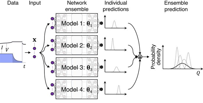
In this flowchart, simple averaging is used to combine the Gaussian-distributed predictions by four independently trained neural networks into an ensemble prediction.

Full size image

The probabilistic prediction shown in Eq. (12) becomes critical when only a small training dataset is available due to a limited experimental budget, technical constraints, and time. The data-size limitation applies to battery aging tests, given that they are typically costly and labor-expensive to run and may last for many months to years, making it practically difficult to test many cells under a wide range of use conditions. A more detailed description of the neural network ensemble method can be found in the original research paper¹⁴³ and a recent tutorial paper on uncertainty quantification of ML models³⁴.

As a final note, neural network ensemble has been traditionally treated as a non-Bayesian method. A more recent study attempted to connect neural network ensemble and Bayesian methods, such as BNN, by providing evidence that combining predictions from independently trained copies of the same neural network architecture approximates the Bayesian model averaging¹⁴⁵. This approximation may be why neural network ensembles produce improved (less overconfident) estimates of the predictive uncertainty on OOD data¹⁴⁶.

SOH estimation

Very few studies attempted to apply neural network ensemble to battery SOH estimation. The most relevant study may be the one done by Shen et al. to estimate cell capacity from a measured sample of the (instantaneous) charge capacity (Q), voltage (V), and current (I) time series during a partial charge cycle¹⁴⁷. These time series measurements were fed as input into multiple deep convolutional neural networks, each of which outputs a capacity estimate. The purpose of ensemble learning was not to quantify predictive uncertainty. Rather, the idea was to combine deterministic capacity estimates from multiple neural networks to derive a final deterministic estimate. The weights assigned to the individual neural networks were optimized and often unequal (i.e., unlike the averaging formulation in Eq. (12). The goal was to ensure prediction accuracy across a wider range of operating conditions than predicting with a single neural network. Ensemble learning, in combination with transfer learning, was validated using a 10-year aging dataset from implantable-grade cells^13,110,111 and the Randomized Battery Usage dataset from the NASA Ames Prognostics Center of Excellence⁸⁶. The work by Shen et al.¹⁴⁷ is a typical example of a general observation: in most SOH estimation studies that use data-driven ML models, prediction accuracy is often the predominant evaluation criterion and, in many cases, the only criterion. We call for coordinated efforts to promote adding the quality of predictive uncertainty as a standard evaluation criterion to the scope of any future study on SOH estimation and health diagnostics and prognostics in general. This quality can be assessed via means well-established in the ML community, such as calibration curves, sparsification curves, and negative log-likelihood, as summarized in³⁴, and those established in the PHM community, such as the α-accuracy zone¹⁴⁸ and β probability¹⁴.

SOH forecasting and RUL prediction

We generally observe that studies on SOH forecasting and RUL prediction recognize the importance of uncertainty quantification much better than studies on SOH estimation. This observation could be attributed to the consensus that predicting a future state is more challenging than estimating the current state and involves an additional uncertainty source of future operating conditions that are often unknown. Outside the battery prognostics field, ensembles of probabilistic neural networks have been applied to solve time series prediction problems for general-purpose prognostics. For example, the bearing prognostics work by Nemani et al.¹⁴⁹ built an ensemble of time series predictors, each being a long short-term memory recurrent neural network with a custom Gaussian output layer. A similar group of authors¹⁵⁰ later applied such an ensemble model for the RUL prediction of Li-ion cells in an open-source aging dataset consisting of 169 LFP cells^27,79. Like the capacity estimation study by Shen et al.¹⁴⁷, the neural network ensemble by Nemani et al.¹⁵⁰ did not adopt simple averaging as the weighting scheme. Instead, the model weights were optimized to minimize the RUL prediction RMSE on a training dataset. It was found that ensemble learning produced uncertainty estimates more representative of prediction errors over single-model learning. This improvement mostly resulted from increased predictive uncertainty and reduced overconfidence in OOD data, attributable to ensemble diversity, i.e., aggregating Gaussian-distributed outputs of the individual models with different means.

It is interesting to see efforts that combine predictions from deterministic ML models to derive a predictive uncertainty estimate. One such example is the capacity forecasting study considering charge and discharge C-rates that vary randomly from one cycle to the next¹⁰³, as also discussed under “RVM applications to battery diagnostics and prognostics SOH estimation”. The authors trained 10 XGBoost models and used the sample standard deviation of the (deterministic) capacity estimates by these models to quantify the predictive uncertainty. The quality of predictive uncertainty was assessed qualitatively by including a sparsification plot that visualized how the prediction accuracy measured by RMSE decreased by incrementally adding test samples with increasing predictive uncertainty. However, without assessment using quantitative metrics such as the expected calibration error and negative log-likelihood, it is unclear how well the predictive uncertainty (known) can approximate the model prediction error (unknown). Nevertheless, an interesting area of exploration could be uncertainty quantification by an emerging family of deterministic methods that only require a single, often deterministic neural network instead of multiple probabilistic neural networks^151,152,153. Benchmarking efforts comparing the more mature probabilistic and emerging deterministic methods will help fill an important knowledge gap in the battery prognostics field.

Counterintuitively, a hybrid method formed by combining a model-based and data-driven method produces lower uncertainty in RUL prediction over the model-based method¹⁵⁴. This uncertainty reduction was achieved by predicting future measurements using an ML model trained on historical data and augmenting the dataset for the model-based method with these predicted future measurements. Given the addition of new data (i.e., the predicted future measurements), uncertainty reduction is not surprising. The lower predictive uncertainty came hand-in-hand with a higher prediction accuracy¹⁵⁴, indicating that the predictive uncertainty was likely a good indicator of the prediction error. This example suggests combining methods or models may increase prediction accuracy (e.g., through data augmentation), together with reduced predictive uncertainty, while combining individual models in a neural network ensemble is not expected to increase prediction accuracy much but yields the benefit of capturing epistemic uncertainty, thereby producing a higher total predictive uncertainty that better represents the prediction error¹⁵⁵.

Sampling methodologies

Unlike Bayesian learning methods, sampling approaches to predictive uncertainty estimation work by evaluating models’ fit to different data subsets via repeated sampling and model training. Bootstrap sampling is a common method of creating many data subsets by repeatedly sampling a dataset. How the sampling is performed (w/wo replacement, stratified, etc.) greatly affects the characteristics of the data subsets and, subsequently, the models’ fit to them¹⁵⁶. Predictive uncertainty is estimated by fitting models of identical architecture to each of the bootstrapped data subsets and aggregating their predictions—plurality vote for classification and averaging for regression. This method, known as bagging and short-hand for “bootstrap aggregating”, is designed to estimate predictive uncertainty by capturing the changes in model predictions due to dataset perturbations induced by the random sampling¹⁵⁷. Bootstrap sampling and bagging (a.k.a. bootstrap aggregating) are explained graphically in Fig. 12. Standard bagging uses models of identical architecture and random sampling with replacement. The subset-to-subset variations in the sample selection produce models with varying optimal parameters, leading to diverse sets of predictions. When the properties of the sampled data subsets closely align with the full dataset, the variation in the fitted models is minimal, and the model prediction intervals tend to be small.

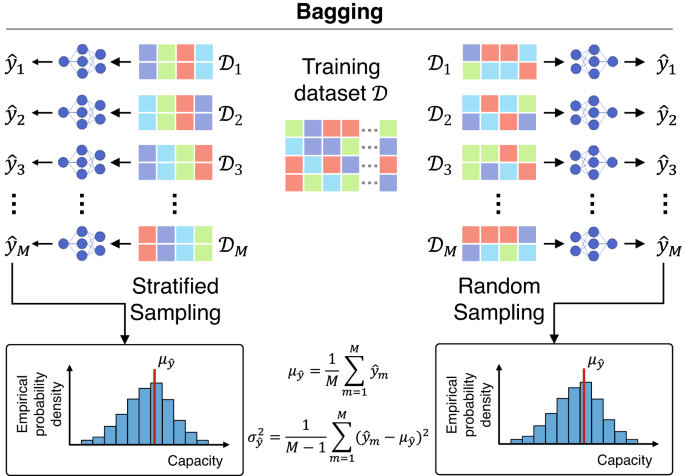
Example ML pipeline for battery capacity estimation using random and stratified sampling bagging methods.

Full size image

Sampling applications to battery diagnostics and prognostics

A common theme among research published on bagging for battery health diagnostics and prognostics is the use of random forest regressors. A random forest regression model is a meta regressor consisting of many binary decision trees that are fit to bootstrap samples of the original dataset¹⁵⁸. The outputs from the many decision trees are averaged to make a mean prediction, and uncertainty can be quantified by examining the spread of the predicted outputs from the individual trees. Random forest models are commonly used in battery health diagnostic and prognostic applications because of their ability to model the nonlinear behavior often observed in battery capacity fade and their probabilistic predictions. Further, random forestmodels have become simple to implement as many publicly available ML model libraries include a random forestimplementation.

SOH estimation

Research on battery capacity estimation using random forestsgenerally focuses on extracting various features from battery capacity-voltage data that correlate strongly with the cell’s capacity. Li et al.¹⁵⁹ conducted aging experiments on two different types of NCM/Gr cells to demonstrate an RF-based capacity estimation algorithm. The researchers extracted IC curves from three different voltage ranges, each spanning roughly 30% of the total SOC range. The researchers found that the voltage range containing a Li+ phase transformation (3.6−3.8 V in NCM/Gr) performed much better than the other two voltage ranges. This was determined to be the case because the phase transformations appear as prominent peaks in the IC curves and the magnitude and location of the peaks are sensitive to the SOH of the cell. The model leveraged the strong correlation between the IC peaks and cell capacity to achieve an average of 1.3% RMSE across the 23 cells. Similar research by Roman et al.¹⁴ used a random forestmodel for capacity estimation as part of an ML pipeline that first extracted 30 features from battery capacity, voltage, and temperature data before down-selecting using a recursive feature elimination scheme. The selected features were then fed to a random forestmodel to estimate the capacity of various cells tested under both standard and fast-charge conditions. The researchers found that while the random forestmodel had the lowest accuracy of those tested, it was overconfident in its predictions of capacity, as indicated by the predictive uncertainty at some samples being overly small relative to the large prediction errors at these samples. Model predictive uncertainty is closely tied to the sample size of the dataset the model is fit to. In the realm of batteries, most datasets are very small in size due to the high costs associated with testing hundreds or thousands of cells. Specific to batteries, assessing the quality of predictive uncertainty quantification (e.g., through uncertainty calibration) is of great importance and should be investigated further³⁴. Other research on battery capacity estimation for second-life applications by Takahashi et al. investigated using a GPR-based bagging approach¹⁶⁰. The researchers first extracted summary statistics, like mean, variance, and inter-quartile-range, from the CC-constant-voltage part of the charging curve and down-selected them to be used as feature inputs to the GPR models. Then, multiple GPR models were fit to bootstrap data subsets to predict battery capacity.

SOH forecasting and RUL prediction

Researchers have also applied bagging to battery capacity forecasting and RUL prediction. Work by Liu et al.¹⁶¹ developed a bagging approach to RUL prediction using monotonic echo state networks to directly predict RUL from an engineered health index. The health index, calculated as the normalized time spent discharging between two fixed voltage limits, was found to work well for direct RUL prediction. However, it is worth noting that such a feature may be unextractable if the operation of the battery cell is such that it rarely discharges completely, as is the case with EVs and other consumer electronics. Research by Jiao et al.¹⁶² investigated a bagging approach to RUL prediction for cells cycled under drive-cycle aging protocols. Their approach leveraged random forestdecision trees that directly mapped to RUL using resistances extracted from EIS spectra along with standard IC and DV curves measured during discharge. They observed that their bagging approach produced a more accurate model than any single model tested, further highlighting the power of bagging.

Notably, sampling methods can also be used with more traditional modeling methods, like standard curve fitting and algebraic reduced-order models, to estimate the uncertainty in model parameters and enable probabilistic trajectory predictions for simple models that are not inherently probabilistic. Algebraic reduced-order models are among the first methods used to model and predict battery capacity fade^3,7. After aging cells in long-term storage and cycling tests, trajectory equations are fit to the normalized cell capacity measurements to model the capacity fade as a function of time and cycles/energy throughput. Trajectory equations of the form Q = 1 − a ⋅ t^b, where Q is cell capacity, t is time, and a and b are fittable parameters, are commonly used because of their flexibility in fitting many different trajectory shapes and their loose ties to describing physical modes of capacity fade. For example, the exponent b = 0.5 is commonly used to model the diffusion-limited process in which capacity is lost with SEI formation on graphite^9,52. In many of the models reported in the literature, the capacity fade rate parameter, a, is typically a function that is time- and cycle-independent and captures the effect of the cell operating conditions, like temperature, DOD, SOC, C-rate, pressure, or any other measurable property, on the observed capacity fade rate. Common function forms used to model cell capacity fade rate are Arrhenius- and Tafel-like in nature^{163,164,165,166,167,168}. Arrhenius relationships are most often used to model the rate of chemical reactions mainly due to the effect of temperature. Similarly, Tafel relationships are used to model the rate of electrochemical reactions considering temperature and the electrochemical potential of materials.

Reduced-order models fit to battery aging datasets are excellent candidates to leverage sampling methods for uncertainty estimation. The various operating conditions and intrinsic cell-to-cell variability (e.g., due to manufacturing tolerances and uncertainty in material properties arising from within-batch and batch-to-batch property variations) produce capacity fade trajectories with varying lifetimes. Researchers Smith, Gasper, and colleagues from the National Renewable Energy Laboratory have published numerous articles on the topic of algebraic life models for forecasting battery SOH and predicting RUL with uncertainty via bagging^52,169,170. In the work by Gasper et al.¹⁶⁹, the researchers compared an ML-identified reduced-order aging model to one identified by a human expert. The human expert-identified model included Arrhenius- and Tafel-like expressions to capture the influence of the operating conditions on cell capacity fade. The ML-identified model was discovered through a symbolic regression method that iteratively tests linear combinations of physical descriptors, like 1/T, 1/T², 1/T³, etc., against the dataset to determine the algebraic form of the capacity fade rate submodel as a function of the aging stressors, a = f(T, SOC, …, etc.). Both the human expert- and ML-identified models were compared in terms of absolute accuracy and predictive uncertainty, where predictive uncertainty was estimated using bagging. By repeatedly sampling the aging dataset and fitting reduced-order models, the authors identified distributions for each model parameter and used the numerous sets of parameters to simulate many capacity trajectories. Predictive uncertainty was then quantified through the spread of the many simulated capacity trajectories, finding that the ML-identified model had roughly half the mean absolute error of the human expert-identified model and showed three times lower predictive uncertainty, with much more accurate predictions of cell capacity. In another paper by Gasper et al.⁵², they explained how uncertainty quantification via bootstrapping is an important tool during the model-form selection phase. The authors went on to demonstrate how model parameter uncertainty can be very large when certain test conditions are left out of the dataset, or when too many fittable parameters are included in the chosen model, making it difficult to identify good values for all model parameters. Altogether, many researchers have demonstrated the value of dataset sampling methods like bagging as excellent tools for enabling uncertainty estimates on traditionally non-probabilistic models and as a means to assess model fitness through estimating model parameter distributions. In the next section, we provide insight into the effects of different bagging approaches for predictive uncertainty estimation for battery health diagnostics and prognostics.

Thoughts on sampling methods for battery data

While bagging is typically performed using standard bootstrap sampling with replacement, varying the sampling strategy can effectively capture different sources of uncertainty in a dataset. Specific to battery health diagnostics and prognostics, stratified sampling can be used to avoid quantifying model predictive uncertainty due to the different operating conditions (or lack thereof) in a battery aging dataset. Standard stratified sampling is performed by first dividing a dataset into various “strata” based on different attributes they share¹⁵⁶. For example, common battery strata are the aging experiment test conditions like temperature, C-rate, and DoD. Then, data subsets are randomly sampled ensuring an equal number of samples come from each stratum. Stratified and random sampling are compared in Fig. 12. The stratified sampling method works well for creating balanced datasets, but is infeasible when a few strata have far fewer samples than the others, as it limits the overall size of the data subsets that can be formed. An alternative approach is to perform unbalanced stratified sampling that ensures at least a single sample from each strata is included. However, depending on the application, this can create models that are biased towards stratum with more samples, and should be done carefully.

Models fit to stratified data subsets will never be expected to extrapolate to unseen operating conditions or other test attributes because at least one battery from each stratum will be included in the data subsets. This effectively eliminates any uncertainties associated with model extrapolation, as all operating conditions are known to the model. Stratified sampling is best used for quantifying the impact of cell-to-cell manufacturing variability, as it is well known that even identically manufactured cells will perform differently when tested under the same conditions^26,27,35,87.

An opposite of stratified sampling is leave-out sampling. This approach to sampling specifically excludes one or many strata from each data subset for the purpose of assessing predictive uncertainty as a function of the strata¹⁷¹. Leave-out sampling is similar to standard cross-validation (CV) in that specific data are left out each iteration, but generally, CV leaves out a much greater number of data each iteration and has fewer total iterations. For example, a typical fivefold CV requires that 20% of the entire dataset be left out each iteration and only five total iterations are performed. In contrast, leave-out sampling typically includes >80% of the entire dataset each iteration and sampling is performed with replacement. Leave-out sampling is useful for determining battery test conditions that are essential to accurate model parameterization. By repeatedly leaving out different strata and assessing model accuracy on a balanced validation dataset, one can map out each stratum’s importance to the model fitting process and identify a subset of strata that are essential for accurate model parameterization. Take, for example, a battery capacity estimation model that gets fit to a dataset containing data ranging from 25 to 50 °C. If asked to predict cell capacity for a sample tested at −20 °C, the model would significantly overpredict the capacity because it had no training data from low-temperature strata to inform it that battery capacity significantly declines at low temperatures due to decreased reaction kinetics and increased charge transfer resistance. In this case, leave-out sampling would be able to identify that low-temperature data is crucial to accurately parameterizing the model, and should be prioritized in future testing.

Understanding and using predictive uncertainty estimates from ML models

Understanding the different types of uncertainty that exist and what they quantify is crucial to properly using probabilistic diagnostic and prognostic models for decision making. Discussed previously in the section “Introduction”, applications like designing serially connected modules or setting warranties are typically concerned with worst-cell behavior. Under these conditions, it is ideal to use a probabilistic ML model that can estimate the full population-wise uncertainty when making predictions, so that the tail-end of the distribution can be accurately quantified.

However, there exist many different probabilistic ML models (see the section “Probabilistic ML techniques and their applications to battery health diagnostics and prognostics”) that each differ in the type of uncertainty they estimate (aleatory, epistemic) and how the uncertainty is quantified (Gaussian, non-parametric, bagging, simple average, etc.). Further, the documentation accompanying the various ML modeling libraries for MATLAB, python, etc., are inconsistent in their documentation making it unclear exactly what uncertainty is being predicted. To this end, this section aims to explain the various types of predictive uncertainty and generally discuss how they can be quantified.

Most publicly available ML models output the total predictive uncertainty—usually a probability mass function for classification or a variance for regression. The total predictive uncertainty can be qualitatively decomposed into aleatory and epistemic uncertainty, each owing to unique uncertainty sources¹⁷².

• Aleatory uncertainty quantifies the inherent stochastic nature of an input, output, or the dependency between the two. It is irreducible by nature and stems from sources like manufacturing process variability, inconsistency of material properties, and variations in experimental test conditions¹⁷³. Aleatory uncertainty, sometimes referred to as data uncertainty, persists in a dataset even if more samples are collected, making it irreducible. Types of aleatory uncertainty most frequently studied in Li-ion batteries are generally electric in nature and include variations in cell capacity, resistance, impedance, and aging. Uncertainty associated with battery performance is considered aleatory uncertainty because testing more cells will not reduce the measured variability since it stems from differences in materials and manufacturing processes. However, testing more samples enables one to more accurately quantify the magnitude of aleatory uncertainty in electrical performance³⁵.

• Epistemic uncertainty arises from an incomplete understanding or model representation of the data and is thus reducible. Common sources of epistemic uncertainty are model simplification, model-form selection, computational assumptions like numerical discretization, and model parameter uncertainties¹⁷⁴. Epistemic uncertainty can generally be further classified into model-form and parameter uncertainty³⁴. Model-form uncertainty arises due to the various simplifications and assumptions made to simplify the model training and inference process. This type of uncertainty is prevalent in battery health diagnostics and prognostics since directly modeling the physics of degradation is largely infeasible, and thus most models assume some simpler form that approximates the observed physics by empirically modeling data, e.g., reduced-order models^51,169. Model-form uncertainty can generally be reduced by increasing model complexity or by directly modeling the underlying physics. Model parameter uncertainty can be reduced by collecting more training data with better accuracy and under more conditions, or by increasing the fidelity of the data measurements.

While it is beneficial to understand the origins of aleatory and epistemic uncertainties, it is difficult to individually quantify them in practice. Instead, the predictive uncertainty output of probabilistic ML models captures the combined effects of aleatory and epistemic uncertainties, quantified as the total predictive uncertainty.

Bayesian models, like RVM (the section “Relevance vector machine”) and GPR (the section “Gaussian process regression”), quantify predictive uncertainty through a posterior mean and covariance matrix. Together, the mean and the diagonal of the covariance matrix can be used to construct a predictive Gaussian distribution for each input sample¹⁷⁵. The predictive uncertainty of GPR typically captures the aleatory uncertainty of the data fairly well, but does not capture model-form and parameter uncertainty since the model is non-parametric in nature. If, for example, a GPR was used with an underlying trend function, it may do a better job at capturing the model-form uncertainty as the final fit considers the fit of the trend function to the data in the presence of noise. Another limitation of Bayesian models is that they inherently assume the spread in the predicted distribution is symmetric about the mean (Gaussian distribution), which may not always be valid depending on the application.

On the other hand, sampling approaches to uncertainty estimation quantify uncertainty through aggregating predictions from the many bootstrapped models and constructing a non-parametric predictive distribution for each input sample. Bagging approaches to uncertainty estimation produce a non-parametric distribution that may or may not be Gaussian. Final predictions are generally made using the mean or median of the predictive distributions. Sampling approaches to uncertainty estimation are flexible making different combinations of sampling methods and models to capture different uncertainties. For example, a neural network ensemble (the section “Neural network ensemble”) will capture aleatory uncertainty and parameter uncertainty well, but will not capture model-form uncertainty since the model structure is not empirically-based and the feature learning process is generally unregulated. On the other hand, an algebraic reduced-order capacity trajectory model that inherently assumes the battery’s capacity fade follows an algebraic trajectory will do a much better job capturing model-form and parameter uncertainty. However, as discussed in the section “SOH forecasting and RUL prediction”, the type of sampling method used (stratified, random, leave-out, etc.) plays a large role in the uncertainty that is captured.

Regardless of the probabilistic ML method used, understanding and quantifying a model’s predictive uncertainty is a crucial step in conveying prediction results. Quantifying model predictive uncertainty is generally done using statistical intervals derived from the predictive distributions. Selecting a statistical interval is application-dependent and depends on the main interest at hand, typically one of quantifying the location of a distribution, the spread of a distribution, or calculating an enclosure interval that captures a portion of the total population. Three main types of statistical intervals exist: confidence interval, prediction interval, and tolerance interval. Explanations of each of these statistical intervals, and their applications to battery health diagnostics and prognostics are outlined below.

• Confidence intervals are used for quantifying the precision of a distribution parameter – typically the mean of a distribution. Confidence intervals are frequently used to calculate an upper and lower bound on a distribution mean where the true value of the mean will fall within the calculated range with specified probability p (usually p = 0.95). Shown in Fig. 13, the confidence interval is the smallest of the three intervals because it captures only the uncertainty in the predicted mean value. The range of the confidence interval is closely related to the model-form uncertainty, and because of this, confidence intervals are useful for assessing model parameter uncertainty. As the sample size approaches infinity, the confidence interval collapses to the true value of the mean.

• Prediction intervals are used for quantifying the range that a single future sample from the population will fall within. For example, after training a GPR model on a small dataset to predict a battery cell’s capacity, one might like to construct an interval that, with a high degree of confidence, will contain the true capacity values for a future cell. Shown in Fig. 13, the prediction interval is wider than the confidence interval because it captures both the uncertainty in the model parameters (epistemic uncertainty) and the data uncertainty (aleatory uncertainty).

• Tolerance intervals are used for quantifying the range that present and all future samples from the population will fall within. In battery cell health diagnostics and prognostics, tolerance intervals are useful for establishing an range that will contain a specified portion of the cell population, providing insight for engineers and manufacturers on the predicted performance of all future cells given the results of limited testing from a small batch. Shown in Fig. 13, the tolerance interval is the widest of the three because it captures the additional uncertainty due to having an incomplete dataset.

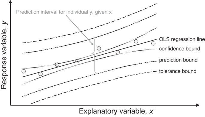
Example illustrating confidence, prediction, and tolerance intervals calculated for an ordinary least squares regressor with a single input feature (x) and target value (y).

Full size image

Calculating a statistical interval differs based on the type of predictive distribution, either parametric (like a Gaussian distribution from RVM or GPR) or non-parametric (like the distribution from a bagging approach or an ensemble model). For parametric distributions like the Gaussian, parametric statistical intervals are straightforward to calculate. The primary interval of interest for Gaussian models is generally a prediction interval. Given we have trained a model on a dataset, prediction intervals tell us with a certain probability where newly tested battery samples will fall. A two-sided 95% prediction interval is calculated as follows:

where (hat{mu }) and (hat{sigma }) are the mean and standard deviation from the predictive distribution, Z is the standard Z-statistic and is equal to 1.96 in this instance, and [PI_l, PI_u] are the lower and upper interval bounds, respectively.

For non-parametric distributions, like those generated from sampling-based methods for uncertainty estimation, the user generally has two options for calculating statistical intervals: (1) approximate the distribution using a known parametric distribution, like Gaussian or log-normal, and calculate the corresponding statistical interval accordingly, or (2) calculate a non-parametric statistical interval. Calculating non-parametric statistical intervals is typically preferred, as assuming a distribution has major implications when trying to understand the tail-ends of the population, e.g., for estimating the worst battery cell performance in a pack. Two-sided non-parametric statistical intervals are not necessarily symmetric, owing to the skewed predictive distribution. Non-parametric statistical intervals are calculated using order statistics, where the upper and lower interval bounds are determined by excluding a calculated number of samples from each tail-end of the predictive distribution and setting the bounds at the lower/upper edges of the remaining samples. The correct number of samples to remove from each end of the predictive distribution is influenced by the desired confidence level p, the number of samples in the predictive distribution N, and, in the case of tolerance intervals, the desired population coverage. The size of the interval is highly dependent on the number of samples in the predictive distribution. However, practically speaking, one can simply increase the number of bootstrap samples to a large number (>1000) to reduce the size of the intervals and achieve higher confidence levels with a narrower interval. Readers interested in calculating one- and two-sided distribution-free statistical intervals are referred to Chapter 5 of the book by Meeker et al.¹⁵⁶.

Diagnostics and prognostics using field data

The general practice in battery diagnostic and prognostic algorithm design is to use cell data collected in the laboratory under predefined load conditions at controlled temperatures (bottom-up approach) and regard battery capacity as the variable of choice to measure battery health, measured periodically via capacity tests¹⁷⁶. Yet, battery capacity is an elusive health metric to estimate when monitoring a battery system used in the field³¹. Battery health diagnostic and prognostic algorithms are deployed to operate on BMSs in real-time and expected to provide accurate health estimates over the entire lifespan of the battery system. One of the main limitations of this approach is that laboratory data can only serve as a small representation of real-world field battery operation and does not reflect application-specific behavior. For instance, in EV applications, battery data will have geographical climate and time-of-day usage dependency, as well as driver-specific behavior³¹. Most importantly, laboratory data do not (and cannot) provide the richness of history-dependent usage trajectories. When SOH algorithms are built from lab data, their predictive ability is challenged upon on-board BMS deployment. This is even more true if the SOH algorithm itself, or any of its components, is based on data-driven ML approaches. Indeed, ML models are limited by the quality of the data used to train them and in terms of how representative the data is of the application at hand. Given the high variability of battery usage in the field, ML-based SOH algorithms developed exclusively from lab data are likely to fail. Moreover, features extracted from lab-generated data and used in data-driven diagnostic and prognostic models will be substantially different, in quality and quantity, from features defined and extracted from real-world driving field data³². Lastly, cell-to-cell heterogeneities are responsible for exacerbated battery system degradation over the battery lifespan but are typically not assessed via lab experiments nor accounted for in current BMSs. In particular, real-time operating conditions contribute to the variability between cells in the form of thermal and aging gradients propagating across the battery pack system, which makes the task of assessing battery health and predicting remaining useful life in real-time more challenging. Such a task cannot solely rely on lab-based offline designed health algorithms.

In light of these challenges, researchers have begun investigating real-world battery usage data for health diagnostics and prognostics. In a recent publication³¹, authors analyzed one-year worth of battery pack data to define health and performance indicators directly learned and extracted from actual driving and charging signal segments. The proposed features were found to be quite different from features previously proposed in the literature to estimate health and predict the remaining lifespan^22,27. The newly extracted features were found to leverage quantities such as resistance calculated during braking or acceleration events and impedance during charging. However, these domain knowledge-based features are also strongly dependent on driving styles, meaning that they would need to be learned on a per-user basis using domain adaptation or similar transfer learning methods. Lu et al.¹⁷⁷ investigated a domain adaptation method to enable seamless transfer of an SOH estimation model from one battery chemistry to another. The researchers were able to train a model that worked well when transferred to a new battery chemistry by extracting domain-invariant features. An algorithm like this one, or similar algorithms proposed in the literature^{178,179,180,181} could conceivably be adapted to enable a model built using lab data to provide good diagnostic and prognostic accuracy in the field.

Other examples of SOH estimation from field data include work by Song et al.¹⁸², where they used a deep neural network to learn relevant features from the historical data of 700 EVs. While not openly available, the dataset was collected by the Shanghai Electric Vehicle Public Data Collecting, Monitoring and Research Center for the purpose of optimizing EV usage in the city and has been used by several other research teams to date^183,184,185. Similar work by She et al.¹⁸⁶ investigated incremental capacity features as input to a radial basis function deep neural network for SOH estimation of electrified city bus battery packs.

Examples of battery health prognostics using field data are more rare since collecting sufficient data for lifetime prediction generally requires many years, since after all, most EVs are warrantied for 8 years and 100,000 mi¹⁸⁷. In our search, we found only a few papers investigating prognostics from field data. Deng et al.¹⁸⁸ built a sequence-to-sequence model with adaptive error correction from a GPR model to predict future capacity fade of 20 EVs operating for over two years using only the first 3 months of data. The model was very accurate with 1.6% average prediction error, but the small size of the dataset (only 20 packs) and similar operating conditions make it difficult to determine the model’s accuracy in various conditions and longer duration. Other work by Zhang et al.¹⁸⁹ used much more data for building a battery prognostic model: two datasets comprising lab aging tests (a few hundred cells) and one dataset comprising data from 7296 PHEVs. The researchers tracked battery aging stressors like SOC, temperature, and throughput using a histogram-based approach and quantified the stressors using summary statistics like mean, variance, skewness, kurtosis, and higher order moments. The extracted feature pool was then reduced using cross-correlation analysis between the features and the target variable of cell capacity. After training a global model on the datasets, the authors implemented an online adjust factor that tunes the global model to an individual battery pack. The adjustment factor is calculated on a rolling basis using the difference between the global model prediction and the observed capacity data, improving accuracy considerably compared to just using the global model for prediction on all vehicles.

Going forward, it will be crucial for academia to collaborate with industry to share data from field units for the purpose of improving diagnostic and prognostic algorithms. Furthermore, developing intelligent data-driven performance forecasting/prediction models for real-time deployment requires re-examining the BMS design paradigm to account for the integration of field operating conditions to allow domain-knowledge learning³³.

Degradation diagnostics

Mentioned earlier in the section “Battery health diagnostic and prognostic problems”, degradation diagnostics is a subproblem of SOH estimation that focuses on methods to non-destructively diagnose internal degradation modes that drive capacity fade and resistance increase⁷¹. Figure 3 gives an overview of the three degradation modes commonly used to quantify cell-level capacity and power fade: loss of active material on the cathode (LAM_PE), the loss of active material on the anode (LAM_NE), and the loss of lithium inventory (LLI). These three degradation modes are commonly used to quantitatively describe the combined effects of certain groups of degradation mechanisms present in the cell, i.e., the degradation modes come from grouping degradation mechanisms based on their resulting effects on cell-level performance. Research by Birkl et al.⁷¹ experimentally verified the effects of each degradation mode on the full-cell OCV curve, providing a quantitative link between the two for the first time. This was achieved by constructing coin cells with electrodes of different sizes to simulate loss of active materials and lithium inventory. The degradation modes were then quantified by using half-cell OCV data to reconstruct the full-cell OCV curve, where the relative position and size of the positive/negative electrode half-cell curves quantify the degradation modes. This work showed that the degradation modes could be accurately quantified by examining full-cell OCV data, albeit through a lengthy and cumbersome curve fitting process that requires access to high-precision measurements of full- and half-cell voltage, current, and capacity during slow and complete cycles.

In light of this, researchers began investigating methods of automating the diagnosis process using various ML-based techniques. In the work by Tian et al.¹⁹⁰, researchers trained a convolution neural network to estimate a cell’s offline OCV curve using data collected from partial charging cycles throughout the day. The trained model could then be used online in place of low-rate full-DOD cycling tests to estimate full-cell OCV, thus enabling and significantly speeding up the process of online degradation diagnostics. Along the same lines, papers^191,192 demonstrated methods of estimating full-cell OCV curves by fitting pristine half-cell OCV data to partial charging curves. While accurate, the methods still required a significant duration of charging data (Schmitt et al.¹⁹² required 20−70% SOC) in order to guarantee accuracy in the range of 2% error on capacity estimation.

While the researchers in refs. ^190,191,192 focused on using cell data to reconstruct OCV curves as an intermediate step in diagnosing degradation modes, the following works aimed to directly correlate cell data with the degradation modes^193,194. Han et al.¹⁹³ proposed using membership functions to quantify the areas under the peak locations of the full-cell differential capacity curve (dQ/dV) and correlating these capacities to loss of lithium inventory and loss of negative electrode materials. Costa et al.¹⁹⁴ focused on transforming the full-cell incremental capacity and differential voltage measurements into a 2D image of the cell’s state that were then fed into a convolution neural network that directly diagnosed the degradation modes. The model was proven to work well on multiple cell chemistries (LFP, NMC, and NCA), achieving an average of 2% error. These works have undoubtedly shown that cell-level data can be directly correlated with internal degradation modes. Yet, few have studied the transferability of the model to new operating conditions outside the datasets used.

The following few works focused on just that: methods of building generalizable ML models for degradation diagnostics^81,195,196. To make the models more generalizable, the following works prioritized incorporating synthetic data from physics-based simulations of cell degradation into their models. Dubarry et al.¹⁹⁵ developed a method relying on an offline database that contained cell full-cell OCV curves and their corresponding degradation modes, simulated using half-cell data from full-cells. The degradation modes of an online cell were quantified by measuring its incremental capacity curve and matching it to the database, interpolating if the curve does not match any of the database entries exactly. While accurate, the database is generally too large to be implemented onboard BMS or other devices. Thelen et al.⁸¹ took a different approach, and instead trained a machine learning model to act as a generalizable aging “database” by training it using a combination of experimental and simulated aging data. Once trained, the model could be used online to directly estimate a cell’s degradation modes using the full-cell incremental capacity curve as input. Other work by Ruan et al.¹⁹⁶ took a similar approach, and trained a deep learning model from a large body of simulated aging data, demonstrating that the degradation modes are inherently correlated, and these correlations can be exploited to improve diagnostic accuracy. Altogether, these methods present a significant leap forward in the ability to non-destructively diagnose unobservable degradation modes in Li-ion batteries.

While all the methods discussed so far have focused on degradation diagnostics using electrical measurements (voltage, current, capacity, etc.), there do exist other methods using alternative data streams. Prosser et al.¹⁹⁷ demonstrated a zero-dimensional cell heat generation model that could accurately diagnose the cell’s degradation modes in-operando. What’s impressive about this work is that the pouch cells were subject to active cooling through the cell tabs, demonstrating the method can be adapted to cells inside modules and packs.

Altogether, the field of degradation diagnostics has come a long way, and we envision these methods and techniques will carry over into battery prognostics, enabling forecasting and life prediction with respect to cell degradation modes in addition to the typical capacity/resistance.

Early life and trajectory prediction

Recognizing the practical value of probabilistic forecasting of SOH evolution and probabilistic predictions of RUL, researchers have recently begun to develop early prediction models with quantified uncertainty. The majority of these papers employ current and voltage information collected early in the battery life to predict RUL or other quantities of interest, as illustrated in Fig. 14. In one of the earliest examples, Fermín-Cueto et al. demonstrated the classification of battery life into categories and the prediction of the number of cycles until the battery capacity exhibited accelerating degradation, termed roll-over or knee-point, both with uncertainty¹⁹⁸. For the classification task, they employed support vector machines to predict whether the cells corresponded to low, middle, or long life categories using data from only the first 3–5 cycles. Class probabilities were estimated using the approach of Platt, where the support vector machine outputs were re-calibrated via logistic regression¹⁹⁹. Knee-points were predicted using the first 50 cycles via RVMs, with conformal prediction intervals for uncertainty. Both tasks employed the 124 LFP cell fast-charging dataset released by Severson et al. with their pioneering 2021 paper²⁷. Several years later, the same group demonstrated predictions of capacity and internal resistance degradation curves with uncertainty via XGBoost (an ensemble decision tree approach) predictions of the knee-onset and knee-point and the capacities (or resistances) at which they occur, in addition to the EOL—again using only the first 50 cycles²⁰⁰.

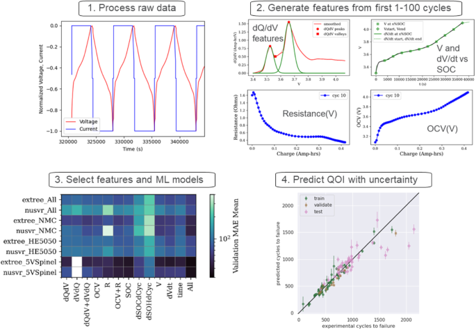
“QOI” in Step 4 stands for quantity of interest. Figure elements borrowed from Paulson et al.⁸⁷

Full size image

As mentioned in the section “SOH forecasting and RUL prediction”, NREL has published several articles employing ML-selected arithmetic relationships to predict changes in battery SOH under a variety of calendar- and cyclic-aging conditions with bootstrapped uncertainty estimates^52,169,170. Notably, this approach provides reasonable extrapolations into later life for a variety of chemistries, cell formats, C-rates, and temperatures due to the semi-physical nature of the models selected by the symbolic regression approach employed and enabling deconvolution of aging mechanisms. This approach does not require preliminary cycling data for a given cell to predict SOH evolution, but does require extensive accelerated testing information spanning conditions for that specific cell type. Techno-economic analyses demonstrated the outsize impact of prediction uncertainty on energy-storage system lifetime.

Rieger et al. demonstrated prognostics of capacity degradation trends for LFP, NMC, and NCA battery chemistries using between 20 and 100 preliminary cycles as context for the prediction²⁰¹. In contrast to previously mentioned approaches, this work employed a deep learning architecture capable of making non-parametric predictions of future degradation trends. Specifically, ensembles of recurrent neural networks were used. Final predictions with uncertainty were obtained by combining ten trajectories sampled from the mean and variance outputs from each of five neural networks trained with randomly initialized weights. Analysis of the uncertainty revealed that the model was slightly overconfident in its predictions, but correctly assigned high uncertainties to longer-lived cells that were less represented in the training set.

Physics-based diagnostics and prognostics

Physics-based models of Li-ion batteries are powerful tools for simulating cell electric, thermal, and mechanical performance. However, they are typically parameterized only on newly manufactured battery cells, relegating them to applications that do not consider cell aging. While in theory, physics-based models can be re-parameterized using data collected from aged cells, doing so would require a large and costly aging test campaign. In light of this, researchers have found other ways to leverage the accuracy and extrapolation capabilities of physics-based models in prognostic frameworks.

One method of leveraging physics-based models for battery health diagnostics and prognostics is to use them as an intermediate step toward SOH estimation or RUL prediction. An example of this approach is illustrated in Fig. 15, where the physics of Li-ion battery degradation is used as an intermediate step to estimate cell capacity and predict cell RUL. Ideally, it is thought that using a physics-based model as an intermediate step helps to include additional information regarding the physics of battery operation and degradation that may not be immediately learnable by a traditional ML model from the available data. Lui et al.²⁰² used this approach to predict the RUL of implantable-grade Li-ion battery cells aged under various temperatures and C-rates. Instead of directly extrapolating the observed capacity-fade trajectories to predict RUL, the researcher first fit a physics-based half-cell model to the measured full-cell OCV curves to obtain rough estimates of the cell’s present active masses (LAM_PE, LAM_NE) and lithium inventory (LLI) (see the section “Battery degradation—modes and mechanisms”). This half-cell model, proposed by Honkura et al.²⁰³ and popularized in later works^204,205, uses experimental data from anode and cathode half-cells to simulate the full-cell voltage vs. capacity curve, typically under a very slow charge/discharge rate (e.g., I < C/20) to approximate the full-cell OCV curve. Then, Lui et al.²⁰² used bounded empirical capacity fade models to extrapolate the degradation parameter values. Estimating cell capacity was then achieved by running the physics-based half-cell model in reverse—inputting the degradation parameters and receiving an estimate of the full-cell OCV curve and the capacity. This method worked well since it was found that many of the degradation parameter trajectories were nearly linear, making their future trajectories easily extrapolated. For many cells in the dataset, the degradation parameter trajectories were nearly linear but combined to produce nonlinear degradation in the full-cell capacity fade curve. Discussed in detail by Attia et al.⁵⁶, degradation modes have various rates of progression, that when combined together in the full-cell environment, interact to produce nonlinear capacity fade and often times knee points in the capacity trajectory. Attia et al.⁵⁶ delve into details regarding the so called “internal state trajectories” of various degradation modes like electrolyte additive depletion, lithium plating, and resistance growth due to active material loss, that drive measurable capacity loss at the cell-level.

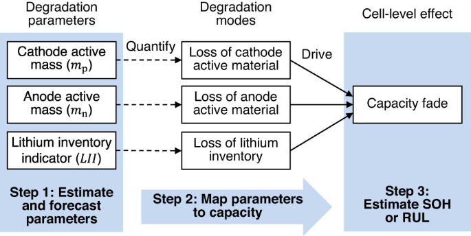
Cell degradation parameters (see the section “Battery degradation — modes and mechanisms”) are estimated and used in a physics-based model to estimate full-cell capacity fade. Based on work of Lui et al.²⁰²

Full size image

Kohtz et al.²⁰⁶ took a similar approach to battery prognostics, which was categorized as a physics-informed ML approach. The researchers used a physics-based model to estimate the thickness of SEI on a Li-ion cell’s anode as an intermediate step to capacity estimation. Instead of using the physics-based model in the prediction process, the authors trained a GPR surrogate model (GPR model #1) to approximate the battery physics and learn the mapping between a partial segment of the cell’s voltage curve and the corresponding SEI thickness for various temperatures, C-rates, and SOH as simulated by the physics-based model. Next, another GPR model (GPR model #2) was trained to learn the mapping between a cell’s SEI thickness and its discharge capacity. The two GPR models are used in series to make a final prediction of cell capacity, first predicting SEI thickness from a partial voltage segment using GPR model #1 and then predicting cell discharge capacity using GPR model #2. Compared to directly predicting cell capacity from a partial voltage segment, the physics-informed approach to capacity estimation showed significantly lower error, mostly attributed to the extra knowledge of SEI thickness infused into the GPR models.

Other methods of using physics-based models for battery prognostics include using the physics-based models to generate simulation data to use for traditional ML model training^81,193,195 and online updating the parameters of the physics-based models using measurements of the cell²⁰⁷. In addition to purely physics-based approaches to prognostics, the field of physics-informed ML has flourished recently with numerous articles leveraging physics knowledge to inform traditional ML approaches for battery health diagnostics^{206,208,209,210} and prognostics^207,211.

Recent work by Pannala et al.²¹² developed a physics-based aging model that linked SEI growth, Li plating, and electrode particle fracture degradation modes to irreversible cell thickness growth, resistance increase, and capacity loss. The method parameterized a single particle model of an NCM111 battery cell and a group of degradation-mode-specific aging models using data collected from RPTs during laboratory aging tests. The model was found to accurately capture and predict changes in cell resistance, capacity, and thickness for a variety of C-rates and DODs. Further, the physics-based nature of the model provides insight into a cell’s remaining lithium inventory (LLI) and remaining positive and negative active electrode materials (LAM_PE, LAM_NE) with aging.

However, we believe there is still a great opportunity to further leverage physics-based models for battery prognostics. In particular, leveraging physics-based models to track and identify battery aging stressors from field data (see the section “Diagnostics and prognostics using field data”) is a novel idea we have yet to see investigated. Further, it is becoming more feasible to deploy lightweight physics-based models on-board EVs as their computing systems are upgraded to accommodate the demand from driver-assistance systems. In online scenarios, fusing sensor data, physics, and ML poses a real solution to accurate battery prognostics in the field.

Second-life applications

In recent years, the market share of EVs has witnessed remarkable exponential growth. Starting from a modest 4% in 2020, EVs now account for 14% of all vehicles sold as of 2022⁴⁷. It is projected that EVs could constitute 18% of total vehicle sales in the near future⁴⁷. The rise in EV adoption holds promising potential for mitigating greenhouse gas emissions in the transportation sector. However, along with these environmental benefits, there arises a pressing concern regarding the exponentially increasing volume of retired Li-ion batteries, imposing a significant challenge to environmental protection and sustainability efforts. While recycling techniques allow for the recovery of valuable battery materials from retired batteries, within the framework of a circular economy, it is widely believed that it is not economically optimal to directly recycle all the retired EV batteries. This is mainly due to the following two primary considerations:

1. 1.

   In the automotive industry, a commonly adopted practice for battery retirement is to replace them when their capacity falls below 80% of their nominal value²¹³. This leaves most retired batteries with a significant portion of their initial capacity that can be utilized by other industries that require less capacity/power performance for energy storage.

2. 2.

   Empirical data show that battery pack degradation often stems from the failure or reduced capacity of a small number of cells within the pack²¹⁴. This means that a majority of cells within a pack tend to have capacities greater than the pack’s EOL condition, making them excellent candidates for reuse in new applications.

The above stipulations have led to immense efforts to integrate remanufacturing and repurposing into the broader circular economy of EV batteries²¹⁵. The ultimate goal is to prolong the service life of retired batteries, affording them a valuable “second life” before they ultimately undergo recycling for raw material collection and disposal.

• Remanufacturing is the process of identifying failed or significantly aged cells within a battery pack and replacing them with new cells or used cells that have been tested and found to meet specifications by OEMs^215,216.

• Repurposing is the practice of giving retired EV batteries a second life in a diverse range of applications. Typical applications include grid energy storage systems, off-grid stationary storage, and recreational vehicles, all of which can function with cells of lesser capacity and power capability.

Roles of probabilistic ML for second-life batteries

Retired EV batteries maintain significant value and functionality when retired at the typical 70-80% initial capacity. However, it remains practically challenging to determine the suitability of a cell/module/pack for remanufacturing or repurposing. This section discusses the future role probabilistic ML methods will play in the evaluation step of a Li-ion battery’s life cycle—with a primary focus on SoH estimation (the section “Background”) and lifetime prediction (the section “Probabilistic ML techniques and their applications to battery health diagnostics and prognostics”). Examples are below.

1. 1.

   Degradation modeling: As detailed in the section “Battery degradation—modes and mechanisms”, Li-ion batteries exhibit numerous aging mechanisms, and the relationship among them is inherently complicated. Given that the safety performance of Li-ion batteries is significantly affected by their aging path and underlying aging mechanisms²¹⁷, comprehending the degradation of EV batteries during their first-life use is crucial in assessing the safety suitability of retired batteries for their intended second-life applications. For instance, capacity degradation may manifest as a loss of Lithium inventory, a phenomenon stemming from various degradation mechanisms such as lithium plating/dendrite, electrolyte decomposition, and SEI decomposition, among others. In cases where dendrite growth is the root cause, growing dendrite could potentially penetrate the separator, causing an internal short circuit, triggering thermal runaway, and, in more severe scenarios, resulting in a fire in the second-life application²¹⁸. Identifying the primary degradation mechanism in the first life can significantly facilitate the safety assessment for subsequent second-life applications. Furthermore, gaining insights into degradation mechanisms from the first-life application could also help predict the potential degradation mechanisms in the second-life application, thus allowing for proactively predicting the service life of the batteries in their second-life applications. The very complicated degradation mechanisms, along with their complex interactions, present substantial hurdles when it comes to degradation modeling and identification. Despite advancements in physics-based degradation modeling, numerous physical phenomena remain unsolved. Leveraging hybrid modeling techniques, which seamlessly integrate probabilistic ML models with physics-based models, offers a promising avenue for addressing these knowledge gaps. Such an approach enables the modeling of un-modeled physics using experimental data, which simultaneously allows for quantifying the predictive uncertainty in the degradation modeling.

   

   Cell SOH assessment for second-life applications.

   Full size image

2. 2.

   SOH estimation: SOH is a widely accepted indicator for battery screening, guiding the selection of suitable second-life applications²¹⁹. When a battery cell/module’s SOH falls significantly below a certain threshold (see Fig. 16), this cell/module can be directly recycled. Conversely, when the SOH remains considerably high, surpassing the EOL criteria for EV applications, the battery can undergo remanufacturing and be repackaged for continued EV use. As depicted in Fig. 16, when the SOH falls within the intermediate range, the battery can be repurposed for second-life applications, such as grid storage and off-grid stationary storage, depending on the battery’s specific SOH level. Therefore, SOH estimation is an indispensable step for second-life applications. As discussed in the section “Probabilistic ML techniques and their applications to battery health diagnostics and prognostics, numerous SOH estimation techniques have been developed in recent years. Among these, data-driven and hybrid approaches have demonstrated their effectiveness in accurately assessing SOH. Specifically, probabilistic ML-based methods, such as the GPR-based approach (see the section “GPR applications to battery diagnostics and prognostics”), provide a distinct advantage. These methods not only produce a mean estimate of the SOH, but they also provide a prediction interval representing the predictive uncertainty. This probabilistic aspect enables decision makers to balance potential benefits and associated risks when choosing the most suitable second-life applications for retired EV batteries. The above discussion does not apply to cases where battery repurposing facilities can directly measure the SOH of a retired EV cell/module, e.g., by running a full charge/discharge cycle, and thus do not require SOH estimation using probabilistic or non-probabilistic ML techniques. These cases are expected to become less common, attributable to the rapidly growing volume of batteries from EVs reaching the end of their life over the next decade. Simultaneously, there is an escalating demand for rapidly assessing battery SOH in mass production settings, where ML techniques with uncertainty quantification capability are likely to play a major role.

3. 3.

   RUL prediction and economic benefits analysis: Let us recall that the primary objective of employing second-life batteries lies in realizing the full economic potential of retired EV batteries. However, the economic viability of selecting retired batteries for specific second-life applications hinges on several factors. These factors include but are not limited to the efficacy of the battery management system, the costs associated with dismantling, and the costs involved in repackaging. Should the expenses of repurposing or remanufacturing surpass the benefits generated by the second-life batteries, it becomes economically unfeasible to extend the service life of retired batteries into their second life. Therefore, a comprehensive analysis of the economic benefits associated with second-life batteries becomes pivotal in evaluating the economic viability of a particular second-life application. A cornerstone technique for conducting such an economic benefits analysis is the RUL prediction of a battery for its second-life application. By analyzing how long the battery can continue to function effectively in the second life, we can assess the long-term benefits or cost savings that second-life batteries can contribute. However, it is worth noting that various uncertainty sources are present in the RUL prediction of second-life batteries, such as degradation mechanism uncertainty, lack of sufficient second-life degradation data, and uncertainty in second-life operation conditions, among others. Given the multifaceted nature of these uncertainty sources, the adoption of probabilistic ML models becomes imperative when predicting RUL for second-life applications. Such models are suitable for handling and quantifying these uncertainty sources, enhancing the accuracy and reliability of RUL prediction for the second-life application. Furthermore, integrating probabilistic RUL prediction into the decision-making process allows decision makers to consider and factor in various uncertainty sources within the economic analysis model when deciding on the second-life application.

Challenges in second-life battery applications

Realizing the economic and environmental potential of second-life batteries faces various challenges. These primary challenges can be summarized as follows (Fig. 17).

1. 1.

   Degradation modeling in the second life: Empirical models, such as stochastic processes and regression models, can be established to predict the first-life degradation of EV batteries based on sensor data acquired from EVs. These empirical models, however, cannot be directly extrapolated for the degradation prediction in the second life, simply because the system may have been reconfigured for the second-life application, and the use conditions in the second life may significantly deviate from those in the first life. Solving this challenge requires establishing strong connections from the first-life field data to the second-life degradation models. Such connections may leverage physics-informed simulation models and the second-life (lab) test data from degradation experiments.

2. 2.

   RUL prediction for second-life applications: The RUL prediction for second-life applications is challenging for several reasons.

   • First, existing prognostic approaches designed for general engineered systems have been successful, in part, in predicting the RULs of these systems. However, these approaches are mostly application-specific and are not robust across different applications, and are thus difficult to be directly applied for lifetime prognostics of retired EV batteries in their second lives.

   • Second, the knee point is where the battery aging transitions from a predominately linear degradation pattern into a nonlinear degradation region with a rapid capacity drop²²⁰. This critical knee point may occur during the first life, as illustrated in Fig. 17, and could also be experienced in second-life application. The exact occurrence time of the knee point is dependent on the cell chemistry, cell design, and usage patterns of the first- and second-life applications. Predicting the knee point is of great importance yet very challenging. Oftentimes, cell manufacturers make efforts in design and manufacturing to ensure an extremely low chance of having a knee point in first-life applications, essentially pushing the knee point into second-life applications. A higher likelihood of having a knee point makes the RUL prediction for the second-life application much more difficult than for the first-life application.

   • Third, as mentioned above, degradation data for second-life applications is usually not sufficient. This poses significant challenges for commonly employed data-driven RUL prediction algorithms.

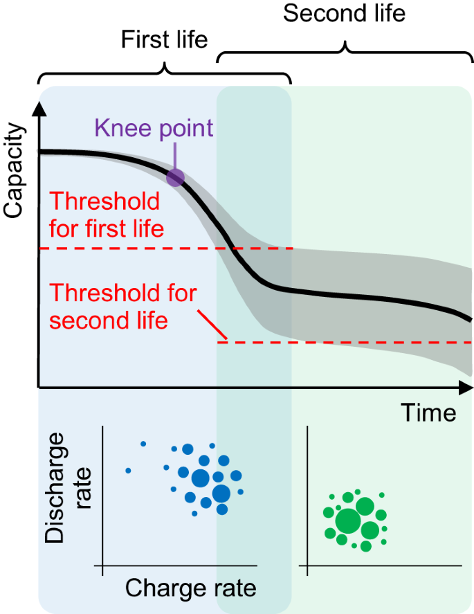
An illustration of an aging trajectory over two lives and a knee point in the second life.

Full size image

Possible solutions to the challenges

We believe the following research directions could provide potential solutions to the aforementioned challenges.

• Physics-informed probabilistic ML for RUL prediction. Physics-informed ML is an emerging concept in the field of failure prognostics²²¹. Incorporating physical laws or domain knowledge into ML models has the potential to substantially reduce the required amount of degradation data for failure prognostics. Furthermore, the synergy between physics-informed ML and the probabilistic ML methods discussed above enables the quantification of the predictive uncertainty due to the lack of sufficient degradation training data in the second-life application. The resulting physics-informed probabilistic ML models may possess the strengths of both learning paradigms. Specifically, physics-informed ML may enhance the extrapolation capability of the degradation model for failure prognostics, while probabilistic ML could quantify the inherent uncertainty in the prediction arising from such extrapolation.

• Battery passport. As pointed out in Thelen et al.²²², an alternative solution lies in the concept of Battery passport, introduced through a public-private collaboration platform called the Global Battery Alliance in November 2020²²³. The passport encompasses all relevant information about the battery from its initial production to its ultimate repurposing or recycling stage. Such a wealth of information could greatly facilitate the estimation of the SOH and prediction of RUL in the second-life application. A similar effort to harmonize battery data collection and reporting standards is the Battery Data Genome²²⁴. By unifying battery data reporting standards and creating more open-access databases, research breakthroughs will be more likely and electrification progress will accelerate.

• Battery digital twins. Similar to the Battery Passport concept, another possible and promising solution is the creation of digital twins tailored to individual batteries²²². The personalized digital replicas of batteries offer the potential for both rapid degradation diagnostics and accurate RUL prediction during their second-life applications.

Aging-aware battery control optimization

Aging-aware battery control optimization aims to regulate battery degradation to either ensure a minimum product lifetime (for ensuring a warranty is met) or extend the product’s lifetime as much as possible, possibly at the expense of the user’s experience²²⁵. Here, we review three main ways in which battery aging can be controlled to extend battery lifetime: adaptive discharging, adaptive charging, and thermal management.

Adaptive discharging

One method of controlling battery degradation and optimizing lifetime is through active discharge control. Limiting the power draw on the battery during discharge can extend the run time and slow the cycling-driven aging. Limiting the discharge power effectively limits the maximum C-rate the battery experiences, which is critical for reducing swelling and diffusion-induced stresses on the electrodes and preventing electrode degradation^26,51. This approach to aging-aware control is shown in Fig. 18, where a power-limited control strategy is compared to standard uncontrolled battery operation. In Fig. 18, the power-limited discharge strategy achieves a much longer run time because the maximum discharge rate is capped. Another effective discharge-based method of reducing battery degradation is by limiting the maximum DOD. Full DOD cycling has been shown to significantly accelerate battery aging, especially on next-generation Si-anode batteries⁵⁹. Limiting the maximum DOD of the battery can prevent significant degradation, thereby prolonging the battery life and, in some cases (when the battery has a shorter expected lifetime than other components), the product that uses the battery as the power source.

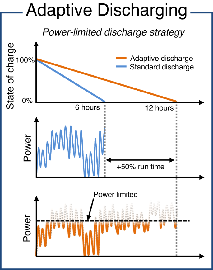
With standard control strategies, power draw is not limited, and run time is uncontrolled (blue curves). With the adaptive discharge control strategy (orange curves), the maximum discharge power is limited to a safe range to extend the run time and reduce cycle-driven battery aging due to high C-rates.

Full size image

Unfortunately, discharge-based methods of regulating battery aging have quickly fallen out of favor with engineers because these methods significantly impact the user experience. Probably the most infamous example of a discharge-based strategy to extend a product’s lifetime was Apple’s attempt to extend the life of users’ iPhones by reducing the microprocessor clock speed via a software update. Reducing the processor clock speed effectively reduced the average power required of the battery, which successfully increased the phone’s run time between charges (or the recharge interval), but at the expense of the phone’s responsiveness to user inputs²²⁶. This practice was extremely unpopular with users and ultimately led to class-action lawsuits against Apple, which were eventually settled in late 2020. This event showed that a majority of users would simply prefer their devices continue to perform like new, even if it means the run time between charges significantly shortens as the battery ages.

Given the challenge of implementing a discharge-based battery aging control strategy without significantly affecting the user experience, engineers and researchers have mostly ceased researching the topic. We see this idea perpetuated in most battery diagnostic and prognostic modeling work reviewed in this paper – most of the works use voltage, capacity, current, and temperature data extracted during charging since battery discharge is mostly uncontrolled and application-dependent. We expect this trend to hold for the foreseeable future and expect future aging-aware control research to focus on charging and thermal management strategies.

Adaptive charging

Depending on the charging speed of interest, charging-based strategies for reducing battery aging can generally be grouped into two categories: slow charging and fast charging.

Slow charging

Research on slow-charging control strategies for reducing battery degradation focuses on a few key competing factors that affect the optimal solution, namely 1) charging during low-cost electricity intervals, 2) charging over long periods to reduce battery self-heating and avoid high temperatures, 3) charging near the end of the available charge time to avoid storage at high SOC, and 4) reducing high-power charging/discharging to grid²²⁷. Hoke et al.²²⁸ used a reduced-order algebraic battery aging model to quickly evaluate the projected lifetime (years to 80% SOH) of four hybrid EV charging strategies: charge on plug in, charge at midnight, charge as late as possible, and charge minimizing electricity costs. Additionally, the charging strategies were evaluated for different charging powers to account for the effect of C-rate on battery aging. The authors showed that their co-optimization method, which minimized both battery degradation and electricity costs, produced projected battery lifetimes far exceeding the other strategies. Notably, their results showed that the strategy of simply waiting to charge until as late as possible in the charging window and using a low charging rate can significantly increase the projected lifetime of the battery. However, the authors did point out that defining the charging window requires knowledge of the user’s behavior, which in many cases needs to be learned from monitoring behavior over a long period. Further, in the context of this study, if the user behavior significantly deviates from the predefined schedule, they may find that their HEV is not fully charged, as the strategy waits until as early in the morning as possible to charge the vehicle. However, with modern phone applications that enable users to control their vehicles (e.g., the Tesla mobile app), it is not inconceivable that a user could manually override the charging strategy to prepare the vehicle for a planned road trip. As battery diagnostic and prognostic models are refined, we expect the details of aging-aware slow-charging optimization will change, but the general premise of balancing battery degradation against electricity costs, user behavior, and other engineering constraints will persist.

Fast charging

In recent years, fast charging has received significant attention because of its role in quickly enabling battery-powered devices to continue normal operation after 15–25 min charging sessions. The technology is significantly important to the continued adoption of EVs by enabling them to “refuel” near the same speeds as traditional internal combustion engines that pump liquid fuel. However, significantly more degradation occurs during fast charging than slow charging due to the extreme C-rates and temperatures the battery cells experience. Under high C-rates, Li-ion batteries are prone to experience lithium plating, which creates unsafe Li-metal dendrites that can cause an internal short-circuit and risk of fire (see the section “Battery degradation – modes and mechanisms”). As a result, research into aging-aware fast charging generally focuses on developing optimal fast-charge profiles to reduce battery degradation from lithium plating using a variety of experimental and simulation-based methods.

An optimal fast-charging profile will balance 1) the charge time (affects the user experience to an extent), 2) the available charger power (modern EV fast chargers are typically limited to 350 kW), 3) battery temperatures (to avoid thermal runaway or maintain EV cabin comfort), and 4) battery aging, among other engineering constraints. Attia et al.⁷⁹ took an experimental approach to fast-charge protocol optimization by cycle aging a large batch of cells (>45 cells) with various 2-step fast charging profiles and then using a Bayesian optimization algorithm to suggest new fast charging protocols for testing, sequentially working towards an optimal fast charging profile for the cell design. Instead of waiting for the cells to reach their EOL, which might take many hundreds of cycles, the researchers used an early life prediction model (see the section “Early life and trajectory prediction”) to predict the lifetimes of the cells after only 100 cycles, increasing the rate at which profiles could be evaluated. The high-throughput experimental testing approach used by Attia et al.⁷⁹ was essentially probing the cell’s lithium-plating limits while simultaneously considering cell self-heating from the high C-rates. The method proved successful, and the authors were able to extend cell life by an average of 180 cycles over previously published fast-charge protocols.

Different from the approach taken by Attia et al.⁷⁹, which focused on optimizing a fast-charging protocol using cell-level aging performance, Konz et al.⁵⁸ looked at fast charging on the component level. They demonstrated a quick and efficient method of experimentally determining a cell’s lithium-plating onset SOC for a given temperature and C-rate by repeatedly cycling graphite half-cells made from the cell’s components. By mapping out the specific C-rates, temperatures, and SOC conditions under which lithium plating occurs in a cell, one can create an optimal fast-charging profile that applies the maximum C-rate without exceeding a margin of safety around the identified lithium plating limit. This approach to fast-charging profile design is very flexible because the optimal profile can be dynamically determined based on the cell’s operating temperature in its intended application. The key advantage of the author’s method over existing ones reported in the literature is that it does not require high precision coulometry equipment and can be done quickly on standard battery cyclers. The method works by performing an SOC-sweep to measure the cell’s coulombic efficiency at a given temperature and C-rate over varied SOCs. If done correctly, one can identify the lithium-plating onset as the point in the CE vs. SOC curve where the CE begins to significantly decline from 100%. A low CE is an indication of irreversible capacity loss due to lithium plating. While the method in Konz et al.⁵⁸ shows promise for significantly improving the speed at which a cell’s lithium-plating limits can be mapped out, the number of tests quickly becomes overwhelming as soon as one wants to adapt the profile as cells age. To capture the effect of cell aging when calculating the optimal fast-charging profile, SOC-sweep cycling tests would need to be performed on aged graphite half-cells, requiring an extensive DOE of aging tests where cells are pulled off at various levels of SOH to conduct SOC-sweeps.

An alternative approach to developing fast-charging profiles considering aging is to use physics-based simulation. In a follow-up paper by Konz et al.²²⁹, the team of researchers conducted a meta-analysis of lithium-plating onset conditions by simulating thousands of unique fast-charging current profiles using a pseudo-2D electrochemical-thermal model of an NMC532/Gr cell. The researchers were able to map out an upper voltage limit over an SOC range that, if exceeded, the cell is likely to experience lithium plating. An example of the lithium-plating voltage limit and a corresponding optimal fast-charging profile is shown in Fig. 19. The main advantage of finding a purely voltage-based lithium-plating limit is its flexibility—voltage is a response to an applied current, making voltage-based lithium-plating limits agnostic to the fast-charging current profile used. To study the impact of aging on the lithium-plating onset, the researchers modified parameters in the electrochemical model to simulate the effects of aging. For example, they simulated loss of active electrode materials (LAM_PE, LAM_NE, see the section “Battery degradation—modes and mechanisms”) by decreasing the value of the active material fraction parameter in the model. Other simulated aging mechanisms included electrode expansion, decreased charge-transfer kinetics, and loss of lithium inventory. The researchers extensively simulated various fast-charging current profiles with P2D model parameters sampled from distributions spanning the expected range corresponding to cells with between 85 and 100% SOH. As expected, the lithium-plating voltage limit was found to decrease with cell aging, meaning it is more likely for aged cells to experience lithium plating if the fast charging profile is not modified to account for cell aging. While the results are certainly interesting, the study was largely exploratory in nature and did not offer many actionable insights for engineers and practitioners since aging was simulated by randomly sampling the P2D model parameters, which largely ignores the path-dependence of aging typically observed in aging tests and from field data 6. While it is profound that the authors were able to demonstrate the lithium-plating voltage limits decrease with cell aging, more work needs to be done to quantify how much the lithium-plating limits need to decrease for a given battery SOH.

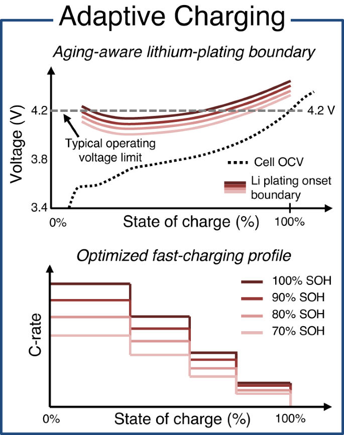
The OCV of an NMC/Gr cell is shown for reference. Bottom, example optimal fast charging profiles for various battery SOHs and designed to charge the cell as fast as possible without the cell voltage exceeding the corresponding lithium-plating voltage limits. Figure based on work by Konz et al.²²⁹.

Full size image

Effectively designing aging-aware fast-charging profiles requires accurately estimating the various degradation mechanisms inside the cell. A combination of capacity, power, and degradation mode estimation⁸¹ is required for characterizing cell SOH and prescribing the proper adjustments to the fast-charging profile. Future research in this area will focus on learning from field battery data uploaded to the cloud how best to adjust fast-charging profiles on a per-user basis—essentially personalizing the charging experience to users individually, as no two batteries will age the same. Research into federated learning methods for training/deploying client-specific ML models will be essential to building optimized aging-aware battery control mechanisms without compromising user’s privacy²³⁰. Additionally, new methods for quickly detecting lithium-plating and designing optimal fast-charging profiles that work for next-generation battery chemistries are needed. Last, new physics-based simulation techniques will need to be developed to more accurately simulate battery aging under real-world conditions, possibly leveraging ML to account for cell aging variability (see the section “Physics-based diagnostics and prognostics”).

Thermal management

The last aging-aware battery control strategy we discuss is thermal management. We highlight thermal management and general thermal modeling of batteries as important future research areas because of their significance in industry-focused product design. Factors like cell/pack packaging, cell form-factor, and regional climate differences (temperature, humidity, pressure, solar radiance) have a great effect on cell temperature within a product, significantly affecting the overall product’s life. In general, most Li-ion batteries are sensitive to temperature and have a small ideal operation window where they perform their best and experience minimum temperature-induced degradation effects, typically in the range 0−40 °C. However, we note that different battery chemistries, particularly next-generation batteries, can have various optimal temperature ranges, and so here we discuss thermal management strategies in a general sense of trying to maintain a lithium-ion battery’s temperature in its optimal range. Figure 20 shows approximate Li-ion battery cycle life as a function of temperature for various charging C-rates. In this example, there exists a stable window between 0 and 35 °C where cycle life remains mostly constant with temperature, indicating the optimal operation window. Below 0 ^∘C, Li-ion batteries are likely to experience lithium plating (see the section “Battery degradation—modes and mechanisms”), and above 40 ^∘C, the rate of SEI formation and other side reactions are significantly increased, decreasing capacity and cycle life rapidly.

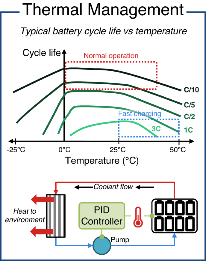
Bottom, an example battery pack cooling strategy that uses liquid coolant to pull heat away from the pack and a heat exchanger to reject the heat to the environment.

Full size image

Generally speaking, active thermal management of Li-ion batteries is only feasible on larger battery-powered systems like grid energy storage, EVs, and HEVs since smaller battery-powered electronic devices like phones and laptops lack the space for air/liquid heat exchangers and compressor systems. Instead, engineers and designers can usually reduce battery temperatures in small electronic devices by simply increasing the energy density of the cells. Given the same power load from the device but with a larger battery, the effective C-rate the cell experiences is lower, reducing self-heating and improving aging performance²³¹.

On large battery systems, battery thermal management is carried out using air, liquids, or refrigerants. Typically, at least one surface of each cell in a pack is exposed, allowing air or liquid to flow over the cell surface, pulling heat away from the cell and dumping it into the surrounding environment. A simple coolant system loop for removing heat from a battery pack and rejecting it to the environment is shown in Fig. 20. Optimizing a thermal control system design and strategy requires understanding how battery aging changes with temperature. Reduced-order aging models, such as from these papers^51,169, are excellent for control strategy optimization since they can simulate battery aging under various temperatures with minimal computational overhead. While average cell temperatures dominate storage aging, minimum and maximum temperatures play a large role in cycling-driven aging. Coupling battery aging models with thermal models to simulate cell internal heating and heat transfer to the coolant is imperative for proper design optimization. Existing research using battery thermal models to devise thermal control strategies suggests that thermal management system and cell co-design will lead to more optimal battery performance in EVs^231,232 by reducing cell temperatures, improving heat transfer away from cells, and shortening fast-charging times. Efficient co-design is best achieved using battery digital twin models^221,222 that couple diagnostic, prognostic, thermal, electrical, and form-factor models to comprehensively simulate multiple battery cells and packs of various designs.

While sufficient battery thermal system optimization and control can be achieved with existing diagnostic and prognostic models, there remain significant challenges that will require further research. Presently, standard practice is to build battery diagnostic and prognostic models for a specific cell design using data collected in the lab. Nearly all the research papers discussed in this review build battery-specific aging models that cannot be used to predict aging for batteries of different designs, packaging configurations, or form-factors. This approach to modeling is inflexible, time-consuming, and not relevant to industry where product design constraints like cell packaging, active cooling, and power requirements change frequently as new features and subsystems are added to the product. For example, Keyser et al.²³¹ simulated pouch cells with different terminal locations (terminals on the same side vs opposite side) and found considerable differences in cell internal heating. Other work by Gasper et al.¹⁷⁰ found that a large-format (>50 Ah) cell’s aspect ratio (area over thickness) significantly affects its thermal resistance and self-heating, demonstrating form factor has a significant effect on cooling system design. These two studies highlight the challenge of building battery diagnostic and prognostic models that can effectively extrapolate to new cell designs, form-factors, and use conditions. Further, regional differences in outdoor air temperatures, solar radiance, and humidity drive aging variability in cells, making uncertainty quantification in simulations essential for drawing accurate conclusions about battery design and control strategies. In light of this, we urge researchers to focus on developing diagnostic and prognostic modeling methods that enable engineers and practitioners to quickly assess the impact of various product design changes on battery aging so that battery-product co-design can be achieved and products can be further optimized. A promising path is physics-based battery diagnostic and prognostic models, like those discussed in the section “Physics-based diagnostics and prognostics”. New battery digital twin models that comprehensively model all aspects of battery performance and aging using a combination of physics and machine learning will be paramount to the future development of battery-powered systems like EVs, consumer electronics, and future aviation efforts^222,233.

Modeling battery degradation is essential for optimizing every aspect of the battery life cycle. From research and development in the lab, to optimizing a fast-charging protocol for aged cells in the field, probabilistic battery diagnostic and prognostic models are core to the continued deployment and success of battery technology. In this work, we reviewed existing and emerging research into probabilistic ML for battery diagnostics and prognostics, emphasizing and highlighting seminal research focusing on the combination of accurate battery health modeling considering uncertainty. Altogether, our review has outlined the great need for more research into uncertainty quantification for battery prognostic models to solve problems related to a lack of data for modeling due to high testing costs, inherent cell-to-cell performance and aging variability stemming from manufacturing and testing limitations, and the sheer severity of consequences arising from poor maintenance and control of battery cells in consumer devices. As research in this area continues to mature, it is envisioned that probabilistic ML models will play a crucial role in creating safe, reliable, and long-lasting battery systems. To this end, we see several long-standing challenges that need to be further investigated by the research community:

1. 1.

   Publicly available battery aging datasets are crucial for accelerating the development of probabilistic battery diagnostic and prognostic models. Existing datasets have been instrumental in furthering research in the field (the section “Publicly available battery aging datasets”), however, they primarily consist of cell-level aging data collected in a lab, largely ignoring the important influence of packaging, cooling systems, and time-varying operating conditions on aging. Collaboration between industry and academia to gather and disseminate high-quality cell/module/pack aging data will be crucial for continued research in the coming years.

2. 2.

   Hybrid ML and physics-based modeling will play a large role in designing the battery-powered systems of tomorrow. There is a great opportunity to develop new physics-based diagnostic and prognostic models and physic-informed ML methods that provide greater accuracy and insight into degradation modes than exist today. We see ML as an important tool for identifying physics-based relationships in battery data collected from the field, and informing the design and development of truly physics-based battery aging models that can provide far greater accuracy than we have today.

3. 3.

   Last, developing coupled thermal, electrical, mechanical, and aging models will be key to optimizing all aspects of cell design. Such models enable the possibility of battery/product co-design where the battery form-factor, packaging, cooling, and control algorithms are all optimized considering a set of unified engineering constraints like cost, volume, weight, energy, operating conditions (regional climate, driving habits), and more. Collaborations between engineering disciplines will be crucial to successfully developing the coupled battery digital twin models of the future.

With future infrastructure and transportation trending toward electric power, batteries will continue to play a pivotal role in our society. The path ahead for future battery research is certainly challenging, but ultimately will be achievable through interdisciplinary collaboration between academic researchers, industry engineers, and regulatory bodies.